| TITLE | SIMPLIS DC/DC DVM Tutorial Part 2 - Advanced Topics |
| APPLIES TO | SIMetrix/SIMPLIS DVM v7.1a |
| KEYWORDS | dvm, tutorial, getting started, ltc3406b, LLC, ISL6527A |
| DESCRIPTION | Advanced topics tutorial for the SIMetrix/SIMPLIS Design Verification Module using the LTC3406B as an example. |
| REVISION | pre-release |
SIMPLIS DVM Tutorial Part 1 - Getting Started
- 1.0 Intro to DVM
- 2.0 Getting Started
- 3.0 Configuring a schematic to use the Full PowerAssist features
- 3.4 Adding Three Terminal Output Load
- 3.5 Adding Full PowerAssist Control
- 3.6 Managing Sources And Loads
- 3.7 Setting Control Parameters
- 3.8 Schematic Configured for Full PowerAssist
- 3.9 Selecting a Built-In Testplan
- 3.10 Viewing Output Report
- 4.0 Adding Curves and Scalars Measurements to the Report
- 5.0 Running the Built-In Efficiency and Line and Load Regulation Testplans
SIMPLIS DVM Tutorial Part 2 - Advanced Topics
- 6.0 Customizing Testplans
- 6.1 Changing Parameter values using the Var and Globalvar Functions
- 6.2 Changing Component Values with the Change Function
- 6.3 Changing the Schematic using Jumpers
- 6.4 The Measurement Testplan Entry
- 6.4.1 Creating Scalar Aliases
- 6.4.2 Promoting Graphs to the Overview Report
- 6.4.3 Promoting Scalars to the Overview Report
- 6.4.4 Suppressing Curve Generation
- 6.4.5 Suppressing Scalar Generation
- 6.4.6 Suppressing Specification Generation
- 6.5 Generating Curves from the Current Simulation Data
- 6.6 Comparing data from previous simulations
- 7.0 Miscellaneous Topics
- 7.1 Pre-Process Scripts
- 7.2 Post-Process and Final-Process Scripts
- 7.3 User-Defined Scalar and Spec Values
- 8.0 Applications
- 8.1 Characterizing Device Level Power Losses
- 8.2 Measuring Control Loop Parameters over Line and Load variation
- 8.3 Summary
SIMPLIS DVM Tutorial Part 2 - Advanced Topics
6.0 Customizing Testplans
DVM Testplans are merely tab-separated text files with a .testplan extension, and may be edited with either a text editor or Microsoft Excel. The syntax is particular to DVM and details can be found at the testplan syntax documentation web page. Some general rules apply:
- Blank lines are ignored.
- Lines starting with the * character are considered comment lines and are ignored.
- Inline comments are not supported. One can comment out a entire line, but not a single field or a portion of a line.
- All non-blank, non-comment lines will be interpreted as a testplan entry, that is, a test to be run.
- Testplans may include a "Header" row. The first entry in this row must start with the three character sequence "
*?@". - Testplans often contain symbolic values - these values are either taken directly from the DVM Control symbol or calculated from values taken from the DVM Control symbol. By using symbolic values the same testplan can be used for a whole class of circuits, rather than just one specific circuit.
- All entries are case insensitive.
The built-in testplans are always a good place to start when building a custom testplan. The entire syncbuck_1in_1out testplan has 129 tests, and we don't have the space to view the entire testplan in this tutorial. Instead we will examine a testplan which includes a representative sample of these 129 tests. In the example testplan shown below, all nine Bode Plot tests from the syncbuck_1in_1out.testplan have been retained. These nine tests cover three input voltages ( Nominal , Minimum , Maximum ) and three loads ( light , 50% , 100% ). Following the Bode Plot tests, we have included a single test of each test type.
There are five columns with column header entries of: analysis, objective, source, load and label. Each non-comment row represents a new test, and entries in each column perform some action either before the simulation executes or after the simulation has completed. Testplans execute from left to right and top to bottom, within the limitations of the system (more on this later ). Each entry in the testplan can be a value, for example the Ac in the analysis column, or a function, like the StepLoad(OUTPUT:1, 50%, 100%) entry in the objective column. The StepLoad(OUTPUT:1, 50%, 100%) function tells the program to "Set the first managed output load to a step load with a initial value of 50% of full load and a final value of 100% of full load." In the following examples we will cover the testplan entries in more detail.
| *** | ||||
|---|---|---|---|---|
| *** A sampling of tests in the syncbuck_1in_1out.testplan | ||||
| *** | ||||
| *?@ analysis | objective | source | load | label |
| *** | ||||
| Ac | BodePlot(OUTPUT:1) | SOURCE(INPUT:1, Nominal) | LOAD(OUTPUT:1, Light) | Ac Analysis|Bode Plot|Vin Nominal|Light Load |
| Ac | BodePlot(OUTPUT:1) | SOURCE(INPUT:1, Nominal) | LOAD(OUTPUT:1, 50%) | Ac Analysis|Bode Plot|Vin Nominal|50% Load |
| Ac | BodePlot(OUTPUT:1) | SOURCE(INPUT:1, Nominal) | LOAD(OUTPUT:1, 100%) | Ac Analysis|Bode Plot|Vin Nominal|100% Load |
| *** | ||||
| Ac | BodePlot(OUTPUT:1) | SOURCE(INPUT:1, Minimum) | LOAD(OUTPUT:1, Light) | Ac Analysis|Bode Plot|Vin Minimum|Light Load |
| Ac | BodePlot(OUTPUT:1) | SOURCE(INPUT:1, Minimum) | LOAD(OUTPUT:1, 50%) | Ac Analysis|Bode Plot|Vin Minimum|50% Load |
| Ac | BodePlot(OUTPUT:1) | SOURCE(INPUT:1, Minimum) | LOAD(OUTPUT:1, 100%) | Ac Analysis|Bode Plot|Vin Minimum|100% Load |
| *** | ||||
| Ac | BodePlot(OUTPUT:1) | SOURCE(INPUT:1, Maximum) | LOAD(OUTPUT:1, Light) | Ac Analysis|Bode Plot|Vin Maximum|Light Load |
| Ac | BodePlot(OUTPUT:1) | SOURCE(INPUT:1, Maximum) | LOAD(OUTPUT:1, 50%) | Ac Analysis|Bode Plot|Vin Maximum|50% Load |
| Ac | BodePlot(OUTPUT:1) | SOURCE(INPUT:1, Maximum) | LOAD(OUTPUT:1, 100%) | Ac Analysis|Bode Plot|Vin Maximum|100% Load |
| *** | ||||
| Ac | ConductedSusceptibility(INPUT:1) | SOURCE(INPUT:1, Nominal) | LOAD(OUTPUT:1, Light) | Ac Analysis|Conducted Susceptibility|Vin Nominal|Light Load |
| *** | ||||
| Ac | Impedance(INPUT:1) | SOURCE(INPUT:1, Minimum) | LOAD(OUTPUT:1, 50%) | Ac Analysis|Input Impedance|Vin Minimum|50% Load |
| *** | ||||
| Ac | Impedance(OUTPUT:1) | SOURCE(INPUT:1, Maximum) | LOAD(OUTPUT:1, 100%) | Ac Analysis|Output Impedance|Vin Maximum|100% Load |
| *** | ||||
| Transient | StepLoad(OUTPUT:1, 50%, 100%) | SOURCE(INPUT:1, Nominal) | Transient|Step Load|Vin Nominal|50% Load to 100% Load | |
| *** | ||||
| Transient | StepLine(INPUT:1, Minimum, Maximum) | LOAD(OUTPUT:1, Light) | Transient|Step Line|Light Load|Vin Minimum to Vin Maximum | |
| *** | ||||
| Transient | Startup(INPUT:1, Maximum) | LOAD(OUTPUT:1, 50%) | Transient|Startup|50% Load|0V to Vin Maximum | |
| *** | ||||
| Transient | ShortCkt(OUTPUT:1, Light) | SOURCE(INPUT:1, Minimum) | Transient|Short Circuit|Vin Minimum|Light Load to Short Circuit | |
| *** | ||||
| Steady-State | Steady-State | SOURCE(INPUT:1, Nominal) | LOAD(OUTPUT:1, 50%) | Steady-State|Steady-State|Vin Nominal|50% Load |
Both the abbreviated and full versions of the sync buck testplan are available in the tutorial download directory:
testplans/6.0_a_sampling_of_the_syncbuck_1in_1out.testplantestplans/dvm_builtin-syncbuck_1in_1out.testplan
6.1 Changing Parameter values using the Var and Globalvar Functions
To create an example testplan showing one method of changing schematic parameter values, we start with the Built-In Sync Buck testplan and remove all but the three Bode Plot tests at nominal input voltage. Whenever you run a built-in testplan, a working copy of the testplan is placed in the schematic's directory, allowing for easy modification. In addition to removing the unneeded tests, we have changed the label. Where the label for the built-in testplan started with "Ac Analysis", the new label starts with "Default Values". A pre-prepared testplan is available in the download zip file.
testplans/6.1_var_start.testplan
| *** | ||||
|---|---|---|---|---|
| *** 6.1_var_start.testplan: starting var testplan for DC/DC tutorial section 6.1 | ||||
| *** | ||||
| *?@ analysis | objective | source | load | label |
| *** | ||||
| Ac | BodePlot(OUTPUT:1) | SOURCE(INPUT:1, Nominal) | LOAD(OUTPUT:1, Light) | Default Values|Bode Plot|Vin Nominal|Light Load |
| Ac | BodePlot(OUTPUT:1) | SOURCE(INPUT:1, Nominal) | LOAD(OUTPUT:1, 50%) | Default Values|Bode Plot|Vin Nominal|50% Load |
| Ac | BodePlot(OUTPUT:1) | SOURCE(INPUT:1, Nominal) | LOAD(OUTPUT:1, 100%) | Default Values|Bode Plot|Vin Nominal|100% Load |
Let's first look at the content of our starting testplan in more detail. The testplan begins with three comment rows, followed by the Header row which starts with the special character sequence *?@. The rows following the Header consist of three valid Bode Plot tests, where the circuit is tested at the nominal input source voltage and for three different load levels ( light , 50%, 100% ). The values 50% and 100% are interpreted as 50% and 100% of full load, respectively. The Output tab of the DVM Control symbol stores the value of full load for this schematic. The symbolic value light represents the lightest load value at which the user believes that the POP analysis will succeed and is also stored on the Output tab of the DVM control symbol.
| Header | Value | Description |
|---|---|---|
| analysis: | AC | Tells the program to expect a valid ac analysis objective in the testplan row. |
| objective: | BodePlot(OUTPUT:1) | Sets the first managed load (OUTPUT:1) to a Bode type load, sets the analysis to run a POP and AC simulation, and measures the scalars for Gain Crossover Frequency, Gain Margin, etc. |
| source: | SOURCE(INPUT:1,value) | Sets the DC value of the first managed input source (INPUT:1). The Nominal, Minimum and Maximum values are taken from the user entries in the DVM Control symbol. Note that the SOURCE(INPUT:1,value) entry doesn't change the subcircuit definition. |
| load: | load(OUTPUT:1,value) | Sets the output load as a percentage of full load, the full load value is taken from the DVM control symbol. |
| label: | varies | A description of the test with "|" delimiters. The label is used to populate the test selection dialog box. Each "|" generates a new branch or sub-level in the test selection dialog. Tests are run in the order in which they appear in the testplan file. Tests are presented in the test selection dialog by an alpha-numeric sort of the label values of each test. |
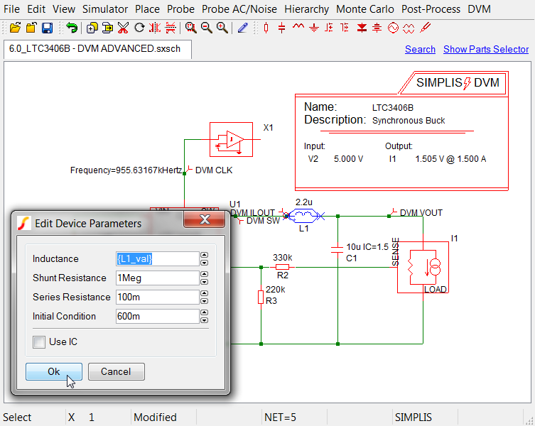
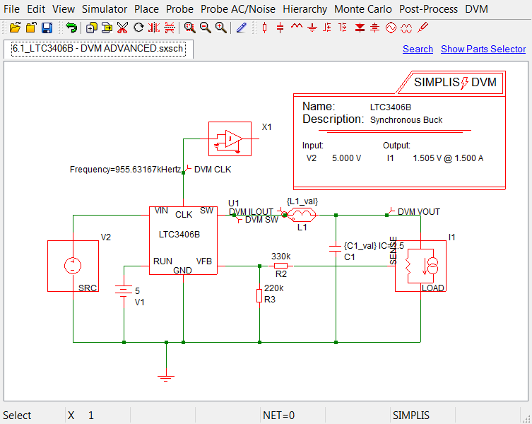
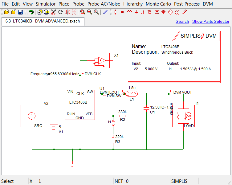
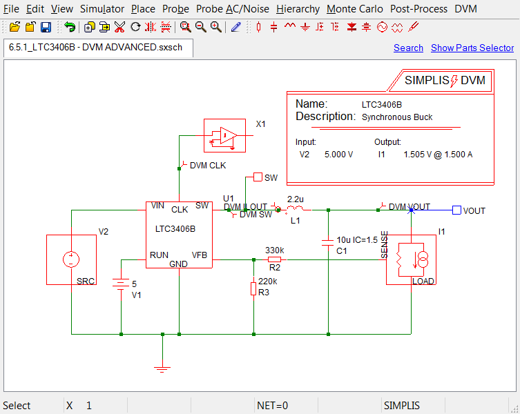
To illustrate how to use the Var and Globalvar statements in a testplan to change schematic parameters, we will use a new schematic which has components which support parametrization. This schematic is electrically equivalent to the schematic in section 4.2. The only change is that the inductor has been replaced with a version which accepts variables. The schematic is available in the download zip file.
LTC3406B/Test Ckts/6.0_LTC3406B - DVM ADVANCED.sxsch

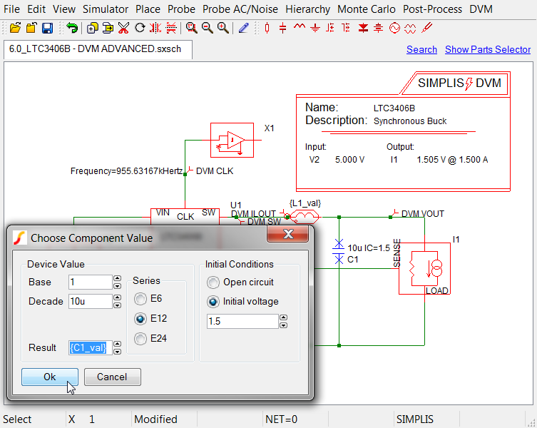
For this example we will parametrize the inductor L1 and capacitor C1 on the top level schematic. To parametrize these two components, double click each one and for the inductor, replace the Inductance value of 2.2u with {L1_val}, and for the capacitor C1 replace the Result value of 10u with {C1_val}. The curly braces { and } tell the program to evaluate the enclosed expression and return a numeric value. This numeric value is used for the simulation, exactly as if it were manually entered as in the earlier schematic examples.
The parametrized schematic is available in the download zip file.
LTC3406B/Test Ckts/6.1_LTC3406B - DVM ADVANCED.sxsch
Once the schematic has been changed to use the variables L1_val and C1_val, we can start modifying the testplan, so that the testplan is used to set the variable values for each test. We first duplicate the three tests, then change the label on the duplicated tests to start with New Values. The modified testplan now has six tests, three with the original, default values, and three which we will populate with new values. The testplan, with added or changed values in red will now looks like this:
| *** | ||||
|---|---|---|---|---|
| *** modified ( 6.1_var_start.testplan ) | ||||
| *** | ||||
| *?@ analysis | objective | source | load | label |
| *** | ||||
| Ac | BodePlot(OUTPUT:1) | SOURCE(INPUT:1, Nominal) | LOAD(OUTPUT:1, Light) | Default Values|Bode Plot|Vin Nominal|Light Load |
| Ac | BodePlot(OUTPUT:1) | SOURCE(INPUT:1, Nominal) | LOAD(OUTPUT:1, 50%) | Default Values|Bode Plot|Vin Nominal|50% Load |
| Ac | BodePlot(OUTPUT:1) | SOURCE(INPUT:1, Nominal) | LOAD(OUTPUT:1, 100%) | Default Values|Bode Plot|Vin Nominal|100% Load |
| *** | ||||
| *** duplicated tests with new test labels | ||||
| *** | ||||
| Ac | BodePlot(OUTPUT:1) | SOURCE(INPUT:1, Nominal) | LOAD(OUTPUT:1, Light) | New Values|Bode Plot|Vin Nominal|Light Load |
| Ac | BodePlot(OUTPUT:1) | SOURCE(INPUT:1, Nominal) | LOAD(OUTPUT:1, 50%) | New Values|Bode Plot|Vin Nominal|50% Load |
| Ac | BodePlot(OUTPUT:1) | SOURCE(INPUT:1, Nominal) | LOAD(OUTPUT:1, 100%) | New Values|Bode Plot|Vin Nominal|100% Load |
Finally, we need to add two new columns to handle the variables L1_val and C1_val. We'll add two new columns, and populate the two column headers with the entries: var(L1_val , 2.2u) and var(C1_val , 10u) respectively.
This function syntax tells the program that the default values for L1_val and C1_val are 2.2u and 10u respectively. For any row in the testplan, DVM will interpret an empty field in either of these columns as the default value, and will write a .VAR statement with the default value in the F11 window of the schematic for that particular test. For any test where the field at this column has a value, DVM will write a .VAR statement into the F11 window of the schematic with the exact text entered in the testplan field. Although the two columns could be added anywhere in the testplan, we'll add them after the objective and before source columns. The final testplan, with added or changed values in red, now looks like this:
| *** | ||||||
|---|---|---|---|---|---|---|
| *** 6.1_var_final.testplan: final var testplan for DC/DC tutorial section 6.1 | ||||||
| *** | ||||||
| *?@ analysis | objective | var(L1_val , 2.2u) | var(C1_val , 10u) | source | load | label |
| *** | ||||||
| Ac | BodePlot(OUTPUT:1) | SOURCE(INPUT:1, Nominal) | LOAD(OUTPUT:1, Light) | Default Values|Bode Plot|Vin Nominal|Light Load | ||
| Ac | BodePlot(OUTPUT:1) | SOURCE(INPUT:1, Nominal) | LOAD(OUTPUT:1, 50%) | Default Values|Bode Plot|Vin Nominal|50% Load | ||
| Ac | BodePlot(OUTPUT:1) | SOURCE(INPUT:1, Nominal) | LOAD(OUTPUT:1, 100%) | Default Values|Bode Plot|Vin Nominal|100% Load | ||
| *** | ||||||
| *** these tests use the new modified values | ||||||
| *** | ||||||
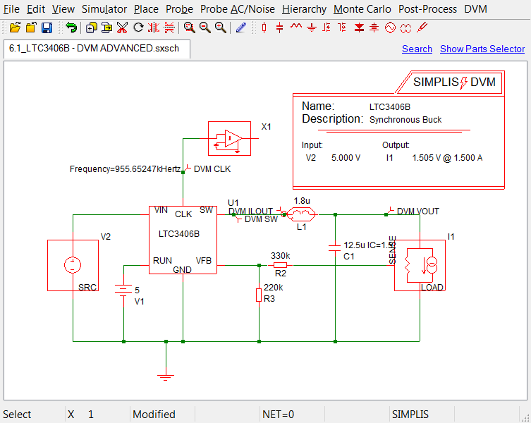
| Ac | BodePlot(OUTPUT:1) | 1.8u | 12.5u | SOURCE(INPUT:1, Nominal) | LOAD(OUTPUT:1, Light) | New Values|Bode Plot|Vin Nominal|Light Load |
| Ac | BodePlot(OUTPUT:1) | 1.8u | 12.5u | SOURCE(INPUT:1, Nominal) | LOAD(OUTPUT:1, 50%) | New Values|Bode Plot|Vin Nominal|50% Load |
| Ac | BodePlot(OUTPUT:1) | 1.8u | 12.5u | SOURCE(INPUT:1, Nominal) | LOAD(OUTPUT:1, 100%) | New Values|Bode Plot|Vin Nominal|100% Load |
This testplan is available in the download zip file:
testplans/6.1_var_final.testplan
The variable statements are written to the schematic's F11 window. Pressing F11 opens this window, which is used for simulator commands, subcircuit models, variables, and the like. The entire contents of the F11 window are added to the beginning of the netlist before the simulation starts. After running one of the default tests, the following variables will be populated in the F11 window.
.VAR L1_val = 2.2u

.VAR C1_val = 10u
Before running this testplan, press F11 to open the F11 window. As the tests execute you will be able to visibly see the .VAR statements as they are written to and deleted from the F11 window.
The Var and Globalvar functions share the exact same syntax. Both will write variable statements to the F11 window. Why use one versus the other? The answer lies in the scope of the functions. A Var entry will only parametrize the top level circuit, lower levels of the hierarchy will not be affected. If, for example, you were to change the capacitor C1 in the opamp schematic LTC3406B_EAMP.sxcmp to have the same {C1_val} value, and ran the simulation you would get an error similar to this:
*** ERRORS REPORTED BY SIMPLIS ***
****************************************
<<<<<<<< Error Message ID: 1038 >>>>>>>>

input file \LTC3406B\Test Ckts\SIMPLIS_Data/6.0_LTC3406B - DVM ADVANCED.deck, line 358:
	C1 6 9 {C1_val} IC=0

A number to represent the value
for `capacitance' is expected at the
location where `{C1_val}' occupies.


*** END SIMPLIS ERROR REPORT ***
What this error is indicates is the variable C1_val was not defined in the netlist for the EAMP subcircuit. To use variables at lower levels of a hierarchical design, you must to use the Globalvar function. If the Var header entries in the testplan 6.1_var_final.testplan are changed to Globalvar entries, the L1_val and C1_val variables will be available at all levels of hierarchy, including the top level. While this feature is very convenient, it can also be dangerous. The global variables being defined will take precedence over any variables defined locally at the hierarchical component level. It is best to define variables locally whenever possible. If using the globalvar function, make certain the variables being defined are not overwriting any local variables. Making the variable names both explicit and unique is a good practice. The testplan using globalvar (modifications in red) will look like this:
| *** | ||||||
|---|---|---|---|---|---|---|
| *** 6.1_globalvar.testplan: globalvar testplan for DC/DC tutorial section 6.1 | ||||||
| *** | ||||||
| *?@ analysis | objective | globalvar(L1_val , 2.2u) | globalvar(C1_val , 10u) | source | load | label |
| *** | ||||||
| Ac | BodePlot(OUTPUT:1) | SOURCE(INPUT:1, Nominal) | LOAD(OUTPUT:1, Light) | Default Values|Bode Plot|Vin Nominal|Light Load | ||
| Ac | BodePlot(OUTPUT:1) | SOURCE(INPUT:1, Nominal) | LOAD(OUTPUT:1, 50%) | Default Values|Bode Plot|Vin Nominal|50% Load | ||
| Ac | BodePlot(OUTPUT:1) | SOURCE(INPUT:1, Nominal) | LOAD(OUTPUT:1, 100%) | Default Values|Bode Plot|Vin Nominal|100% Load | ||
| *** | ||||||
| *** these tests use the new modified values | ||||||
| *** | ||||||
| Ac | BodePlot(OUTPUT:1) | 1.8u | 12.5u | SOURCE(INPUT:1, Nominal) | LOAD(OUTPUT:1, Light) | New Values|Bode Plot|Vin Nominal|Light Load |
| Ac | BodePlot(OUTPUT:1) | 1.8u | 12.5u | SOURCE(INPUT:1, Nominal) | LOAD(OUTPUT:1, 50%) | New Values|Bode Plot|Vin Nominal|50% Load |
| Ac | BodePlot(OUTPUT:1) | 1.8u | 12.5u | SOURCE(INPUT:1, Nominal) | LOAD(OUTPUT:1, 100%) | New Values|Bode Plot|Vin Nominal|100% Load |
testplans/6.1_globalvar.testplan
6.2 Changing Component Values with the Change Function
In section 6.1 we learned how to add variables to the symbol properties, and then use the Var and Globalvar functions to set the variable values. What about changing the schematic symbol values directly? This is exactly what the Change function does. Once you understand the Var and Globalvar syntax, you'll be ready to use the change function - as it shares a similar syntax to the Var and Globalvar functions. Let's use the Change function to produce an testplan equivalent to the 6.1_globalvar.testplan but with the values changed directly on the schematic.
Changing values on most top level symbols is easy. Starting with the testplans/6.1_globalvar.testplan , simply edit the header row, replacing the two globalvar entries with change entries. The arguments inside the parentheses also change - instead of setting the variable values L1_val and C1_val, we are supplying the reference designator of the symbol whose value we desire to change, e.g. L1 and C1. The modified testplan (modifications in red) will look like this.
| *** | ||||||
|---|---|---|---|---|---|---|
| *** 6.2_change_top_level_values.testplan: change testplan for DC/DC tutorial section 6.2 | ||||||
| *** | ||||||
| *?@ analysis | objective | change(L1 , 2.2u) | change(C1 , 10u) | source | load | label |
| *** | ||||||
| Ac | BodePlot(OUTPUT:1) | SOURCE(INPUT:1, Nominal) | LOAD(OUTPUT:1, Light) | Default Values|Bode Plot|Vin Nominal|Light Load | ||
| Ac | BodePlot(OUTPUT:1) | SOURCE(INPUT:1, Nominal) | LOAD(OUTPUT:1, 50%) | Default Values|Bode Plot|Vin Nominal|50% Load | ||
| Ac | BodePlot(OUTPUT:1) | SOURCE(INPUT:1, Nominal) | LOAD(OUTPUT:1, 100%) | Default Values|Bode Plot|Vin Nominal|100% Load | ||
| *** | ||||||
| *** these tests use the new modified values | ||||||
| *** | ||||||
| Ac | BodePlot(OUTPUT:1) | 1.8u | 12.5u | SOURCE(INPUT:1, Nominal) | LOAD(OUTPUT:1, Light) | New Values|Bode Plot|Vin Nominal|Light Load |
| Ac | BodePlot(OUTPUT:1) | 1.8u | 12.5u | SOURCE(INPUT:1, Nominal) | LOAD(OUTPUT:1, 50%) | New Values|Bode Plot|Vin Nominal|50% Load |
| Ac | BodePlot(OUTPUT:1) | 1.8u | 12.5u | SOURCE(INPUT:1, Nominal) | LOAD(OUTPUT:1, 100%) | New Values|Bode Plot|Vin Nominal|100% Load |
This testplan is available in the download directory:
testplans/6.2_change_top_level_values.testplan
When one of the New Values tests from the 6.2_change_top_level_values.testplan testplan is run on the schematic:
LTC3406B/Test Ckts/6.1_LTC3406B - DVM ADVANCED.sxsch
the schematic values will change from the variable names {L1_val} and {C1_val} to the values in the testplan, namely 1.8u and 12.5u. The variable statements in the F11 window will also be deleted, and the schematic will be configured as follows:
A schematic saved at this point is available in the tutorial download file:
LTC3406B/Test Ckts/6.2_LTC3406B - DVM ADVANCED.sxsch
What about changing properties other than the inductor or capacitor value? Both symbols and hierarchical components can have multiple properties, for example L1 is a lossy inductor defined as a subcircuit. The lossy inductor model has properties for the shunt and series resistances as well as the inductance. The property names and values can be seen by clicking the context menu option ( Edit/Add Properties... ).
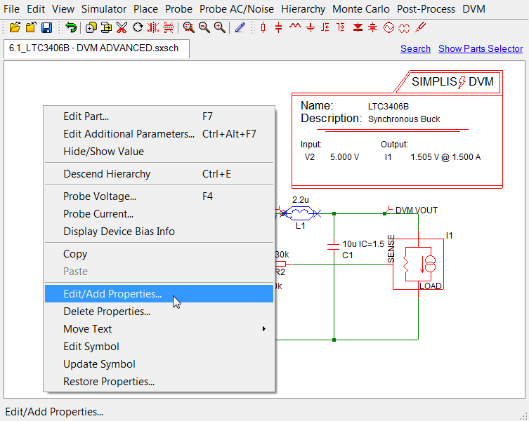
The dialog box shows each property name and it's corresponding value listed in a two column format.

Properties in the Name column can be changed by referencing the property address in 1st argument of the change function. The property address is simply the reference designator and the property name separated with a ".". For example, to change the RSERIES value, the address is L1.RSERIES. In the following testplan (modifications in red), the RSERIES property of L1 is changed from the default value of 100m to a new value of 50m.
| *** | ||||||
|---|---|---|---|---|---|---|
| *** 6.2_change_property_address.testplan: property address change testplan for DC/DC tutorial section 6.2 | ||||||
| *** | ||||||
| *?@ analysis | objective | change(L1.RSERIES , 100m) | change(C1 , 10u) | source | load | label |
| *** | ||||||
| Ac | BodePlot(OUTPUT:1) | SOURCE(INPUT:1, Nominal) | LOAD(OUTPUT:1, Light) | Default Values|Bode Plot|Vin Nominal|Light Load | ||
| Ac | BodePlot(OUTPUT:1) | SOURCE(INPUT:1, Nominal) | LOAD(OUTPUT:1, 50%) | Default Values|Bode Plot|Vin Nominal|50% Load | ||
| Ac | BodePlot(OUTPUT:1) | SOURCE(INPUT:1, Nominal) | LOAD(OUTPUT:1, 100%) | Default Values|Bode Plot|Vin Nominal|100% Load | ||
| *** | ||||||
| *** these tests use the new modified values | ||||||
| *** | ||||||
| Ac | BodePlot(OUTPUT:1) | 50m | 12.5u | SOURCE(INPUT:1, Nominal) | LOAD(OUTPUT:1, Light) | New Values|Bode Plot|Vin Nominal|Light Load |
| Ac | BodePlot(OUTPUT:1) | 50m | 12.5u | SOURCE(INPUT:1, Nominal) | LOAD(OUTPUT:1, 50%) | New Values|Bode Plot|Vin Nominal|50% Load |
| Ac | BodePlot(OUTPUT:1) | 50m | 12.5u | SOURCE(INPUT:1, Nominal) | LOAD(OUTPUT:1, 100%) | New Values|Bode Plot|Vin Nominal|100% Load |
This testplan is available in the download directory:
testplans/6.2_change_property_address.testplan
What about changing properties on schematic symbols at lower levels of a hierarchical design? In section 6.1 we used the globalvar function to set global variables - these variables will be available in all levels of hierarchy. As it turns out, the change function can also modify symbol property values in the hierarchy. To do so, we need to extend the property address system to include the hierarchical location of the symbol. This is called the hierarchical property address.
Symbols in the hierarchy have a unique hierarchical property address. The hierarchical property address is simply a list of reference designators, separated by the "." character. The actual property to be changed is added to the end of the list of reference designators. Note this is exactly the same syntax we used for the top level L1.RSERIES example, in that case, there were no additional reference designators before L1, therefore the entire hierarchical property address was L1.RSERIES.
To demonstrate how the change function can change hierarchical component values, let's start with the schematic:
LTC3406B/Test Ckts/6.2_LTC3406B - DVM ADVANCED.sxsch
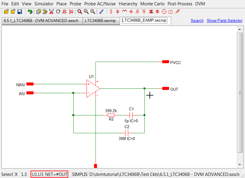
First descend into the hierarchy by selecting the LTC3406B, and pressing the keyboard shortcut ( Ctrl-e ), or use the right-click menu item ( Descend Hierarchy ). This symbol has reference designator U1.
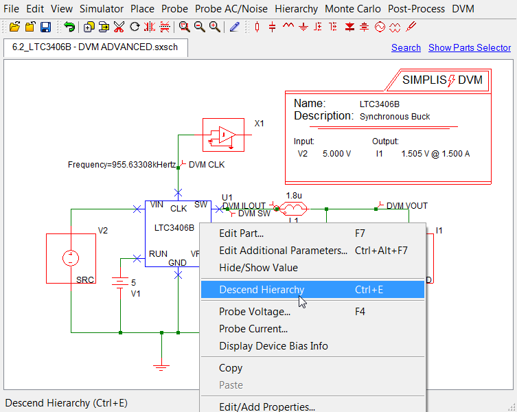
This action descends into the first level of the LTC3406B. Next, descend into the the error amplifier U3 by selecting the EAMP symbol and pressing the keyboard shortcut ( Ctrl-e ), or use the right-click menu item ( Descend Hierarchy ).

We are now at the level where we want to change a component value. To get to this level, we first descended into U1, then into U3. On the lower left hand portion of the schematic window, the hierarchical path to the currently displayed schematic is listed (we highlighted this with a red box):
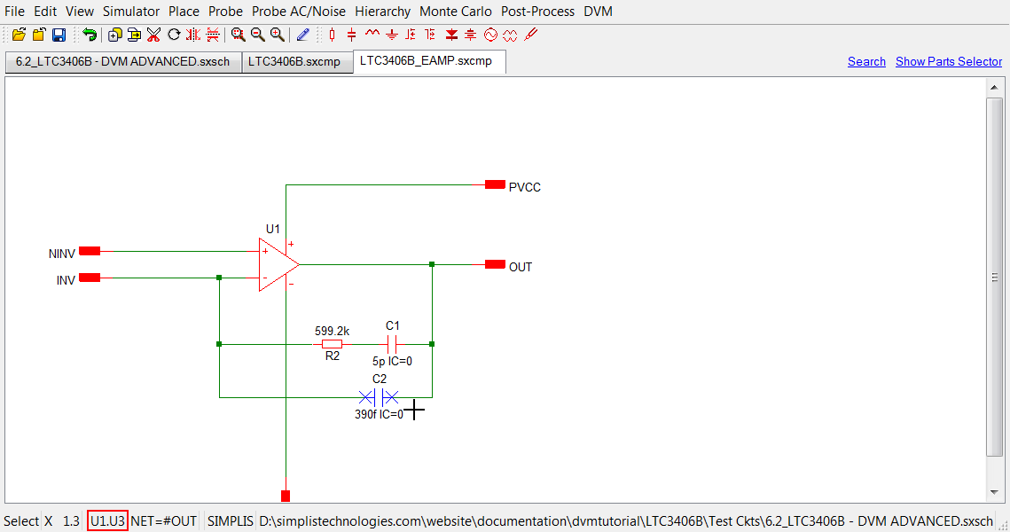
We will use this path to build our hierarchical property address. To change the value of C2 on this schematic, we first take the hierarchical path to this schematic, U1.U3, then add the component which we wish to change to the end with a "." separator: U1.U3.C2. Our final testplan (modifications in red) for this section demonstrates both the top level property address L1.RSERIES, and the hierarchical property address U1.U3.C2.
| *** | ||||||
|---|---|---|---|---|---|---|
| *** 6.2_change_hierarchical_property_address.testplan: hierarchical property address change testplan for DC/DC tutorial section 6.2 | ||||||
| *** | ||||||
| *?@ analysis | objective | change(L1.RSERIES , 100m) | change(U1.U3.C2 , 390f) | source | load | label |
| *** | ||||||
| Ac | BodePlot(OUTPUT:1) | SOURCE(INPUT:1, Nominal) | LOAD(OUTPUT:1, Light) | Default Values|Bode Plot|Vin Nominal|Light Load | ||
| Ac | BodePlot(OUTPUT:1) | SOURCE(INPUT:1, Nominal) | LOAD(OUTPUT:1, 50%) | Default Values|Bode Plot|Vin Nominal|50% Load | ||
| Ac | BodePlot(OUTPUT:1) | SOURCE(INPUT:1, Nominal) | LOAD(OUTPUT:1, 100%) | Default Values|Bode Plot|Vin Nominal|100% Load | ||
| *** | ||||||
| *** | ||||||
| *** | ||||||
| Ac | BodePlot(OUTPUT:1) | 50m | 450f | SOURCE(INPUT:1, Nominal) | LOAD(OUTPUT:1, Light) | New Values|Bode Plot|Vin Nominal|Light Load |
| Ac | BodePlot(OUTPUT:1) | 50m | 450f | SOURCE(INPUT:1, Nominal) | LOAD(OUTPUT:1, 50%) | New Values|Bode Plot|Vin Nominal|50% Load |
| Ac | BodePlot(OUTPUT:1) | 50m | 450f | SOURCE(INPUT:1, Nominal) | LOAD(OUTPUT:1, 100%) | New Values|Bode Plot|Vin Nominal|100% Load |
This testplan is available in the download directory:
testplans/6.2_change_hierarchical_property_address.testplan
When this testplan is run on the schematic:
LTC3406B/Test Ckts/6.2_LTC3406B - DVM ADVANCED.sxsch
You will see that as DVM executes each test, DVM will descend into U1, then into U3, and change the component value for C2. The program then ascends to the top level and executes the simulation.
!!! Warning !!!
Because the schematic values are changed directly using the change function, you should always have a back-up copy of the schematic, in case the changed values render the circuit inoperable. Also if you save a DVM schematic upon completion of a DVM testplan, the schematic will be saved with the components values of the current ( changed ) state of the circuit. Exactly what changes get made to your schematic depends on which tests were run.6.3 Changing the Schematic using Jumpers
In sections 6.1 and 6.2, we change schematic component values using the var, globalvar, and change functions. What if we need to make schematic topology changes that cannot be easily implemented by changing the value of components? This is where the schematic jumpers come in quite handy.
The jumper symbols have either one or two positions and can have up to 64 poles. Through the testplan, the positions of the jumpers can be changed on a test-by-test basis, which offers quite a bit of flexibility in schematic configuration. To manipulate jumpers from the testplan, add a column with the Header entry of jumper. Then in each test row use open( reference designator list ) or close( reference designator list ) to open and close jumpers, where reference designator list is a comma separated list of jumper reference designators. For two position jumpers, the options are open, pos1, and pos2.
To demonstrate the schematic jumpers, we will start with the schematic from section 6.2:
LTC3406B/Test Ckts/6.2_LTC3406B - DVM ADVANCED.sxsch
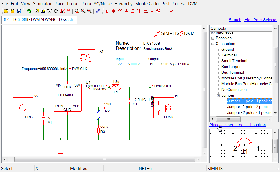
We take this schematic and add a single position jumper symbol to open the connection to the feedback resistor R3. When the R3 path is open, the output voltage will regulate at the reference voltage of the LTC3406B. To place the jumper symbol, use the parts selector category Connectors|Jumper|Jumper - 1 pole - 1 position. While placing the jumper, the symbol may be rotated by pressing F5 and flipped by pressing F6.
The correctly configured schematic shown below is available in the download directory at:
LTC3406B/Test Ckts/6.3_LTC3406B - DVM ADVANCED.sxsch
To control the jumpers from the testplan, we need a single extra column with the Header entry jumper. In the first three test rows, we add close( J1 ) for the default case which has a regulated output voltage of 1.505V. In the new tests, we use open( J1 ) to set the output voltage to 600mV. Additionally, we have changed the test labels to reflect the output voltage regulation set-point. Our jumper manipulation testplan will look like the following, with entries added to or modified from the default testplan in red:
| *** | |||||
|---|---|---|---|---|---|
| *** 6.3_jumpers.testplan: jumper testplan for DC/DC tutorial section 6.3 | |||||
| *** | |||||
| *?@ analysis | objective | jumper | source | load | label |
| *** | |||||
| Ac | BodePlot(OUTPUT:1) | close( J1 ) | SOURCE(INPUT:1, Nominal) | LOAD(OUTPUT:1, Light) | VOUT=1.505V|Bode Plot|Vin Nominal|Light Load |
| Ac | BodePlot(OUTPUT:1) | close( J1 ) | SOURCE(INPUT:1, Nominal) | LOAD(OUTPUT:1, 50%) | VOUT=1.505V|Bode Plot|Vin Nominal|50% Load |
| Ac | BodePlot(OUTPUT:1) | close( J1 ) | SOURCE(INPUT:1, Nominal) | LOAD(OUTPUT:1, 100%) | VOUT=1.505V|Bode Plot|Vin Nominal|100% Load |
| *** | |||||
| *** the jumper position sets the output voltage to 0.6V | |||||
| *** | |||||
| Ac | BodePlot(OUTPUT:1) | open( J1 ) | SOURCE(INPUT:1, Maximum) | LOAD(OUTPUT:1, Light) | VOUT=0.6V|Bode Plot|Vin Maximum|Light Load |
| Ac | BodePlot(OUTPUT:1) | open( J1 ) | SOURCE(INPUT:1, Maximum) | LOAD(OUTPUT:1, 50%) | VOUT=0.6V|Bode Plot|Vin Maximum|50% Load |
| Ac | BodePlot(OUTPUT:1) | open( J1 ) | SOURCE(INPUT:1, Maximum) | LOAD(OUTPUT:1, 100%) | VOUT=0.6V|Bode Plot|Vin Maximum|100% Load |
The already configured testplan is available in the download directory at:
testplans/6.3_jumpers.testplan
After executing a single test from each group of tests, the overview report shows the test with the default output voltage of 1.505V passes the test specifications. The new test with an output voltage of 600mV test fails as expected, since we did not change the output voltage specifications in the Control symbol when we used the jumper to change the output voltage set point.
Note that any number of jumpers can be used for schematic configuration. Multiple jumper-headed columns can be used, although in theory a maximum of three columns are needed - one each for the three possible jumper positions. Multiple jumper reference designators can be added to the reference designator list with comma separators as described in the testplan syntax.
6.4 The Measurement Testplan Entry
The measurement testplan entry allows general purpose results post-processing of simulation data. A number of functions can be entered in a measurement column, and these are the focus of the balance of this section.
6.4.1 Creating Scalar Aliases
A number of scalar measurements are made automatically after each DVM simulation test. In many cases the names for these scalars are determined by the probes on the schematic and as a result are the same for every test. For example, when a Bode Plot test Objective is run, the scalars gain_crossover_frequency, gain_margin, and phase_margin are generated. Often we would like to compare one set of scalar measurements with the same scalar results from other simulation tests run under different operating conditions. To do so, it is advantageous to rename the scalars from each set of tests to reflect the distinguishing test conditions. This becomes quite important when we consider generating curves from the scalar measurements in section: 6.6.2 CreateXYScalarPlot function. To demonstrate the scalar aliasing function, we will start with the testplan from section 6.3.
testplans/6.3_jumpers.testplan
We take this testplan and add three measurement columns for our alias entries. In the column fields for the nominal output voltage tests we will put the following three alias functions:
alias(gain_margin,gain_margin_nom)alias(phase_margin,phase_margin_nom)alias(gain_crossover_freq,gain_crossover_freq_nom)
alias(gain_margin,gain_margin_600mV)alias(phase_margin,phase_margin_600mV)alias(gain_crossover_freq,gain_crossover_freq_600mV)
alias function merely copies the value to a new scalar name. Our alias testplan, with added entries shown in red will look like:
| *** | ||||||||
|---|---|---|---|---|---|---|---|---|
| *** 6.4.1_alias.testplan: alias testplan for DC/DC tutorial section 6.4.1 | ||||||||
| *** | ||||||||
| *?@ analysis | objective | jumper | measurement | measurement | measurement | source | load | label |
| *** | ||||||||
| Ac | BodePlot(OUTPUT:1) | close( J1 ) | alias(gain_margin,gain_margin_nom) | alias(phase_margin,phase_margin_nom) | alias(gain_crossover_freq,gain_crossover_freq_nom) | SOURCE(INPUT:1, Nominal) | LOAD(OUTPUT:1, Light) | VOUT=1.505V|Bode Plot|Vin Nominal|Light Load |
| Ac | BodePlot(OUTPUT:1) | close( J1 ) | alias(gain_margin,gain_margin_nom) | alias(phase_margin,phase_margin_nom) | alias(gain_crossover_freq,gain_crossover_freq_nom) | SOURCE(INPUT:1, Nominal) | LOAD(OUTPUT:1, 50%) | VOUT=1.505V|Bode Plot|Vin Nominal|90% Load |
| Ac | BodePlot(OUTPUT:1) | close( J1 ) | alias(gain_margin,gain_margin_nom) | alias(phase_margin,phase_margin_nom) | alias(gain_crossover_freq,gain_crossover_freq_nom) | SOURCE(INPUT:1, Nominal) | LOAD(OUTPUT:1, 100%) | VOUT=1.505V|Bode Plot|Vin Nominal|100% Load |
| *** | ||||||||
| *** the jumper position sets the output voltage to 0.6V | ||||||||
| *** | ||||||||
| Ac | BodePlot(OUTPUT:1) | open( J1 ) | alias(gain_margin,gain_margin_600mV) | alias(phase_margin,phase_margin_600mV) | alias(gain_crossover_freq,gain_crossover_freq_600mV) | SOURCE(INPUT:1, Maximum) | LOAD(OUTPUT:1, Light) | VOUT=0.6V|Bode Plot|Vin Maximum|Light Load |
| Ac | BodePlot(OUTPUT:1) | open( J1 ) | alias(gain_margin,gain_margin_600mV) | alias(phase_margin,phase_margin_600mV) | alias(gain_crossover_freq,gain_crossover_freq_600mV) | SOURCE(INPUT:1, Maximum) | LOAD(OUTPUT:1, 50%) | VOUT=0.6V|Bode Plot|Vin Maximum|50% Load |
| Ac | BodePlot(OUTPUT:1) | open( J1 ) | alias(gain_margin,gain_margin_600mV) | alias(phase_margin,phase_margin_600mV) | alias(gain_crossover_freq,gain_crossover_freq_600mV) | SOURCE(INPUT:1, Maximum) | LOAD(OUTPUT:1, 100%) | VOUT=0.6V|Bode Plot|Vin Maximum|100% Load |
The already configured testplan is available in the download directory at:
testplans/6.4.1_alias.testplan
When this testplan is run on the schematic from section 6.3:
LTC3406B/Test Ckts/6.3_LTC3406B - DVM ADVANCED.sxsch
the new scalar names appear in the test report.
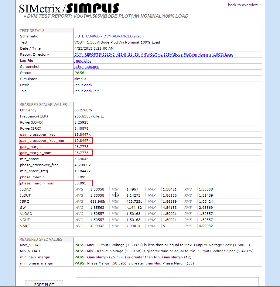
A quick note about scalar names - some auto-generated scalars are reformatted when presented in the html version of the report. Currently this is limited to the table of values with entries for the AVG, MIN, MAX, RMS and Pk2Pk values. The actual scalar names which you will need to use in the alias function for these scalars will be:
Avg(scalarname)Min(scalarname)Max(scalarname)Rms(scalarname)Pk2Pk(scalarname)
scalarname is the name of the scalar in the test report. In the test report above, if we wanted to alias the average output voltage from this test, we would add an entry to the testplan that might look like:
alias(Avg(VOUT),avg_vout_nom)
6.4.2 Promoting Graphs to the Overview Report
In section 5.1 we ran the built-in efficiency testplan and saw the efficiency summary graph was placed on the overview test report. The graph itself was created during the Generate Efficiency Curves test, and the measurement function, PromoteGraph was used to copy the graph from the Generate Efficiency Curves test to the overview report. Although in this case, only one graph was placed on the overview report, any number of graphs can be added and the ordering can be defined as well. There is also provision for renaming the graphs on the overview report. To implement this functionality, there are four versions of the PromoteGraph function. Only the first argument is required, the three optional arguments allow for more flexibility:
PromoteGraph( graphname )PromoteGraph( graphname , weight)PromoteGraph( graphname , weight , use_approximate_name)PromoteGraph( graphname , weight , use_approximate_name , overview_graphname)
BODE PLOT:
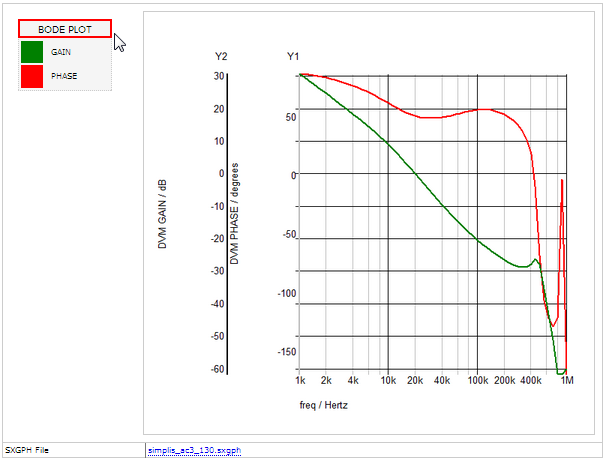
Note this is an approximate graph name, as the full graph name, which can be found in the report.txt file is DVM Bode Plot#log#ac. In order to use the approximate name, the third argument, use_approximate_name should be the number 1, as this tells the program to find a match to the approximate graph name in the available graph names. For most SIMPLIS simulations, the approximate graph name can be used.
A weighting system orders overview graphs from first to last by highest to lowest numerical weight. The ordering or weight argument is optional, and if not used, a default weight of 1 will be assigned. Finally, the optional overview_graphname will rename the graph on the overview report. The overview_graphname is also optional.
To show how the PromoteGraph function works, we'll promote the Bode Plot and output load voltage and current graphs to the overview report. We will start with the last testplan from section 6.4.1.
testplans/6.4.1_alias.testplan
Next, we add two more measurement columns, retaining the three which already exist. In these measurement columns put the appropriate PromoteGraph functions. As there are four PromoteGraph functions, we'll use one of each in this example. The order of the promoted overview graphs will be the same as the function order shown below. The first two functions will promote the graphs from a nominal output voltage test, the third and fourth functions from a test with the output voltage set to 600mV.
- PromoteGraph( BODE PLOT, 100 , 1 , Bode Plot Nominal Vout )
- PromoteGraph( LOAD , 90 , 1 )
- PromoteGraph( DVM BODE PLOT#log#ac , 80 )
- PromoteGraph( DVM LOAD#pop )
The testplan prepared for promoting the graphs to the overview report is shown below. The added entries are shown in red font.
| *** | ||||||||||
|---|---|---|---|---|---|---|---|---|---|---|
| *** 6.4.2_promotegraph.testplan: promotegraph testplan for DC/DC tutorial section 6.4.2 | ||||||||||
| *** | ||||||||||
| *?@ analysis | objective | jumper | measurement | measurement | measurement | measurement | measurement | source | load | label |
| *** | ||||||||||
| Ac | BodePlot(OUTPUT:1) | close( J1 ) | alias(gain_margin,gain_margin_nom) | alias(phase_margin,phase_margin_nom) | alias(gain_crossover_freq,gain_crossover_freq_nom) | SOURCE(INPUT:1, Nominal) | LOAD(OUTPUT:1, Light) | VOUT=1.505V|Bode Plot|Vin Nominal|Light Load | ||
| Ac | BodePlot(OUTPUT:1) | close( J1 ) | PromoteGraph( BODE PLOT, 100 , 1 , Bode Plot Nominal Vout ) | PromoteGraph( LOAD , 90 , 1 ) | alias(gain_margin,gain_margin_nom) | alias(phase_margin,phase_margin_nom) | alias(gain_crossover_freq,gain_crossover_freq_nom) | SOURCE(INPUT:1, Nominal) | LOAD(OUTPUT:1, 50%) | VOUT=1.505V|Bode Plot|Vin Nominal|90% Load |
| Ac | BodePlot(OUTPUT:1) | close( J1 ) | alias(gain_margin,gain_margin_nom) | alias(phase_margin,phase_margin_nom) | alias(gain_crossover_freq,gain_crossover_freq_nom) | SOURCE(INPUT:1, Nominal) | LOAD(OUTPUT:1, 100%) | VOUT=1.505V|Bode Plot|Vin Nominal|100% Load | ||
| *** | ||||||||||
| *** the jumper position sets the output voltage to 0.6V | ||||||||||
| *** | ||||||||||
| Ac | BodePlot(OUTPUT:1) | open( J1 ) | alias(gain_margin,gain_margin_600mV) | alias(phase_margin,phase_margin_600mV) | alias(gain_crossover_freq,gain_crossover_freq_600mV) | SOURCE(INPUT:1, Maximum) | LOAD(OUTPUT:1, Light) | VOUT=0.6V|Bode Plot|Vin Maximum|Light Load | ||
| Ac | BodePlot(OUTPUT:1) | open( J1 ) | PromoteGraph( DVM BODE PLOT#log#ac , 80 ) | PromoteGraph( DVM LOAD#pop ) | alias(gain_margin,gain_margin_600mV) | alias(phase_margin,phase_margin_600mV) | alias(gain_crossover_freq,gain_crossover_freq_600mV) | SOURCE(INPUT:1, Maximum) | LOAD(OUTPUT:1, 50%) | VOUT=0.6V|Bode Plot|Vin Maximum|50% Load |
| Ac | BodePlot(OUTPUT:1) | open( J1 ) | alias(gain_margin,gain_margin_600mV) | alias(phase_margin,phase_margin_600mV) | alias(gain_crossover_freq,gain_crossover_freq_600mV) | SOURCE(INPUT:1, Maximum) | LOAD(OUTPUT:1, 100%) | VOUT=0.6V|Bode Plot|Vin Maximum|100% Load | ||
This testplan is available in the tutorial download directory.
testplans/6.4.2_promotegraph.testplan
When we open the overview report, the Bode Plot is the first graph and has been renamed BODE PLOT NOMINAL VOUT, this was promoted from a nominal output voltage test. The next graph, titled LOAD is the corresponding POP output voltage and current waveforms for the nominal output voltage case. The third graph, titled BODE PLOT is from the 600mV output voltage test. The final graph shows the POP output voltage and current waveforms for the 600mV Bode Plot test . Note the graph title is LOAD, and is therefore the same graph title as the second graph on the overview report. As this might cause some confusion, we recommend users rename graphs with helpful names for the report readers as they are promoted to the overview report with the PromoteGraph function.
A final note of caution - using the approximate graph name may match multiple graphs. An example of this is using this promotegraph function on converters with multiple outputs.
PromoteGraph( LOAD , 3 , 1 )
This will match all load graphs, assuming the loads were automatically named by DVM as LOAD1, LOAD2, etc. If there is ever any doubt about which graph is being promoted, the full name can be found in the report.txt file and used with the use_approximate_name set to 0.
6.4.3 Promoting Scalars to the Overview Report
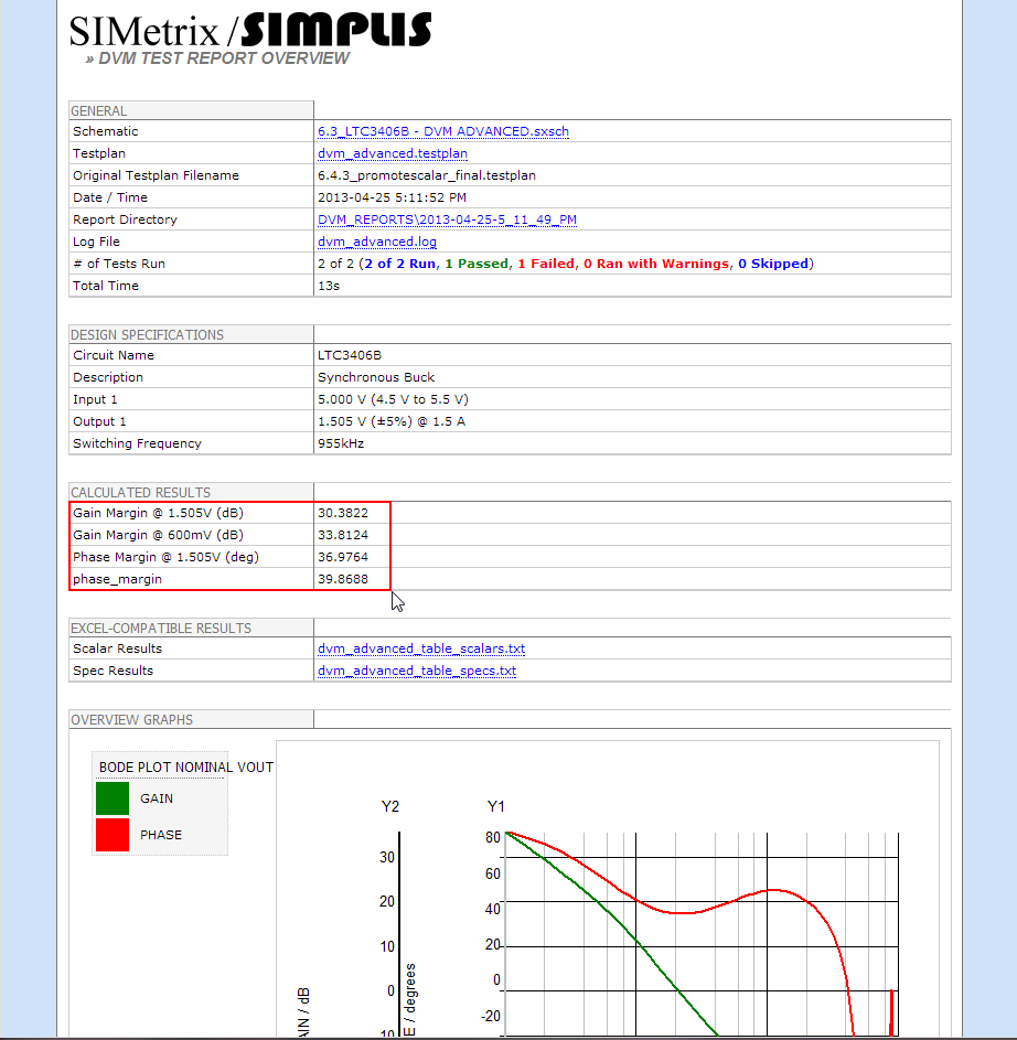
In section 5.2 Line and Load Regulation, we saw the line and load regulation scalar values were automatically placed on the overview report in the CALCULATED RESULTS section. Individual scalars from a test can be copied to the overview report with the PromoteScalar testplan function. Any number of scalars can be promoted by using multiple PromoteScalar calls, and there is a provision for renaming the scalars on the overview report as well. For this function to work properly, the original scalarname must not contain spaces, but the overview scalarname may contain spaces. This helps to clarify what the scalar value represents on the overview report, as the auto-generated scalar name is often not as descriptive as we would like.
To demonstrate the PromoteScalar function, we revisit the testplan from section 6.4.2 Promoting Graphs to the Overview Report. Starting with the testplan from that section, remove the alias columns entirely and add two measurement columns after the jumper column. The resulting testplan will have four measurement columns, two for PromoteGraph and two for PromoteScalar entries. An already prepared starting testplan is included in the tutorial download file with the additional columns highlighted in red.
6.4.3_promotescalars_start.testplan
| *** | ||||||||||
|---|---|---|---|---|---|---|---|---|---|---|
| *** 6.4.3_promotescalars_start.testplan: promotescalar testplan for DC/DC tutorial section 6.4.3 | ||||||||||
| *** | ||||||||||
| *?@ analysis | objective | jumper | measurement | measurement | measurement | measurement | source | load | label | |
| *** | ||||||||||
| Ac | BodePlot(OUTPUT:1) | close( J1 ) | SOURCE(INPUT:1, Nominal) | LOAD(OUTPUT:1, Light) | VOUT=1.505V|Bode Plot|Vin Nominal|Light Load | |||||
| Ac | BodePlot(OUTPUT:1) | close( J1 ) | PromoteGraph( BODE PLOT, 100 , 1 , Bode Plot Nominal Vout ) | PromoteGraph( LOAD , 90 , 1 ) | SOURCE(INPUT:1, Nominal) | LOAD(OUTPUT:1, 50%) | VOUT=1.505V|Bode Plot|Vin Nominal|90% Load | |||
| Ac | BodePlot(OUTPUT:1) | close( J1 ) | SOURCE(INPUT:1, Nominal) | LOAD(OUTPUT:1, 100%) | VOUT=1.505V|Bode Plot|Vin Nominal|100% Load | |||||
| *** | ||||||||||
| *** the jumper position sets the output voltage to 0.6V | ||||||||||
| *** | ||||||||||
| Ac | BodePlot(OUTPUT:1) | open( J1 ) | SOURCE(INPUT:1, Maximum) | LOAD(OUTPUT:1, Light) | VOUT=0.6V|Bode Plot|Vin Maximum|Light Load | |||||
| Ac | BodePlot(OUTPUT:1) | open( J1 ) | PromoteGraph( DVM BODE PLOT#log#ac , 80 ) | PromoteGraph( DVM LOAD#pop ) | SOURCE(INPUT:1, Maximum) | LOAD(OUTPUT:1, 50%) | VOUT=0.6V|Bode Plot|Vin Maximum|50% Load | |||
| Ac | BodePlot(OUTPUT:1) | open( J1 ) | SOURCE(INPUT:1, Maximum) | LOAD(OUTPUT:1, 100%) | VOUT=0.6V|Bode Plot|Vin Maximum|100% Load | |||||
Starting with this testplan, we can add our PromoteScalar entries in the first two measurement columns. Since we promoted the Bode Plot graphs to the overview, it would make sense to also promote the scalar values for Gain Margin and Phase Margin from each test. This will allow a quick visual inspection of both the graphs and the scalar results from those graphs, all on the overview report.
The Gain Margin and Phase Margin scalars are named gain_margin and phase_margin respectively. Let's promote the nominal output voltage scalars as:
PromoteScalar( gain_margin , Gain Margin @ 1.505V (dB))PromoteScalar( phase_margin , Phase Margin @ 1.505V (deg))
Then, mostly to see the PromoteScalar function at work without the overview scalar renamed, we'll make two PromoteScalar entries, one with a renamed scalar and one without.
PromoteScalar( gain_margin , Gain Margin @ 600mV (dB))PromoteScalar( phase_margin )
Our final testplan, ready to be run now looks like:
| *** | ||||||||||
|---|---|---|---|---|---|---|---|---|---|---|
| *** 6.4.3_promotescalars_final.testplan: promotescalar testplan for DC/DC tutorial section 6.4.3 | ||||||||||
| *** | ||||||||||
| *?@ analysis | objective | jumper | measurement | measurement | measurement | measurement | source | load | label | |
| *** | ||||||||||
| Ac | BodePlot(OUTPUT:1) | close( J1 ) | SOURCE(INPUT:1, Nominal) | LOAD(OUTPUT:1, Light) | VOUT=1.505V|Bode Plot|Vin Nominal|Light Load | |||||
| Ac | BodePlot(OUTPUT:1) | close( J1 ) | PromoteScalar( gain_margin , Gain Margin @ 1.505V (dB)) | PromoteScalar( phase_margin , Phase Margin @ 1.505V (deg)) | PromoteGraph( BODE PLOT, 100 , 1 , Bode Plot Nominal Vout ) | PromoteGraph( LOAD , 90 , 1 ) | SOURCE(INPUT:1, Nominal) | LOAD(OUTPUT:1, 50%) | VOUT=1.505V|Bode Plot|Vin Nominal|90% Load | |
| Ac | BodePlot(OUTPUT:1) | close( J1 ) | SOURCE(INPUT:1, Nominal) | LOAD(OUTPUT:1, 100%) | VOUT=1.505V|Bode Plot|Vin Nominal|100% Load | |||||
| *** | ||||||||||
| *** the jumper position sets the output voltage to 0.6V | ||||||||||
| *** | ||||||||||
| Ac | BodePlot(OUTPUT:1) | open( J1 ) | SOURCE(INPUT:1, Maximum) | LOAD(OUTPUT:1, Light) | VOUT=0.6V|Bode Plot|Vin Maximum|Light Load | |||||
| Ac | BodePlot(OUTPUT:1) | open( J1 ) | PromoteScalar( gain_margin , Gain Margin @ 600mV (dB)) | PromoteScalar( phase_margin ) | PromoteGraph( DVM BODE PLOT#log#ac , 80 ) | PromoteGraph( DVM LOAD#pop ) | SOURCE(INPUT:1, Maximum) | LOAD(OUTPUT:1, 50%) | VOUT=0.6V|Bode Plot|Vin Maximum|50% Load | |
| Ac | BodePlot(OUTPUT:1) | open( J1 ) | SOURCE(INPUT:1, Maximum) | LOAD(OUTPUT:1, 100%) | VOUT=0.6V|Bode Plot|Vin Maximum|100% Load | |||||
Let's open the jumper schematic from section 6.3 and run the two 50% Load tests at the two different output voltages.
LTC3406B/Test Ckts/6.3_LTC3406B - DVM ADVANCED.sxsch
In the resulting overview test report, we can see all four scalar values with new and descriptive names for three. The single phase_margin scalar is from the 600mV test and wasn't renamed. The short time it takes to rename the scalars in the testplan appears to be well rewarded.
6.4.4 Suppressing Curve Generation
There may be times when curves are auto-generated which we don't want to show up in our test reports. A DVM testplan function NoCurves exists to suppress either named curves or all curves for a managed source or load.
The nocurves function takes a single argument, and that argument can be one of three types:
- A reference designator of a DVM source or load, e.g.
V2orI1 - A symbolic reference designator, e.g
OUTPUT:norINPUT:n - A actual curvename, e.g.
DVM ILOAD
.sxgph. Valid NoCurves function calls include:
NoCurves( OUTPUT:1 )NoCurves( INPUT:1 )NoCurves( V2 )NoCurves( DVM ILOAD )
NoCurves function.
6.4.5 Suppressing Scalar Generation
There may be instances where auto-generated scalars are not required and we desire to remove these from the test report. The NoScalars function is provided to accomplish this.
The NoScalars function takes a single argument, the reference designator of the source or load for which scalars are not desired. The source or load reference designator can either:
- A reference designator of a DVM source or load, e.g.
V2orI1 - A symbolic reference designator, e.g
OUTPUT:norINPUT:n
NoScalar function calls are:
NoScalars( OUTPUT:1 )NoScalars( INPUT:1 )NoScalars( V2 )NoScalars( I1 )
6.4.6 Suppressing Specification Generation
In section 6.3 Changing the Schematic using Jumpers, we modified the schematic with a jumper symbol, thereby setting the output voltage to 600mV. As a result, the test fails to meet specifications, because the output voltage is considerably out of range. For cases like this, DVM has an option to disable specification checking using the NoSpecs function. The syntax for the NoSpecs function is identical to the NoScalars function. A few examples are:
NoSpecs( OUTPUT:1 )NoSpecs( I1 )
As an example of the three measurement functions NoCurves, NoScalars, and NoSpecs, let's start with the testplan from 6.3 Changing the Schematic using Jumpers.
testplans/6.3_jumpers.testplan
We'll add three measurement columns and in each we will add the three functions:
NoCurves( DVM ILOAD )NoScalars( INPUT:1 )NoSpecs( OUTPUT:1 )
| *** | ||||||||
|---|---|---|---|---|---|---|---|---|
| *** 6.4.6_nocurves_noscalars_nospecs.testplan: nocurves, noscalars, nospecs testplan for DC/DC tutorial section 6.4.6 | ||||||||
| *** | ||||||||
| *?@ analysis | objective | jumper | measurement | measurement | measurement | source | load | label |
| *** | ||||||||
| Ac | BodePlot(OUTPUT:1) | close( J1 ) | SOURCE(INPUT:1, Nominal) | LOAD(OUTPUT:1, Light) | VOUT=1.505V|Bode Plot|Vin Nominal|Light Load | |||
| Ac | BodePlot(OUTPUT:1) | close( J1 ) | SOURCE(INPUT:1, Nominal) | LOAD(OUTPUT:1, 50%) | VOUT=1.505V|Bode Plot|Vin Nominal|50% Load | |||
| Ac | BodePlot(OUTPUT:1) | close( J1 ) | SOURCE(INPUT:1, Nominal) | LOAD(OUTPUT:1, 100%) | VOUT=1.505V|Bode Plot|Vin Nominal|100% Load | |||
| *** | ||||||||
| *** these tests are retained from the original 6.3_jumpers.testplan | ||||||||
| *** | ||||||||
| Ac | BodePlot(OUTPUT:1) | open( J1 ) | SOURCE(INPUT:1, Maximum) | LOAD(OUTPUT:1, Light) | VOUT=0.6V|Bode Plot|Vin Maximum|Light Load | |||
| Ac | BodePlot(OUTPUT:1) | open( J1 ) | SOURCE(INPUT:1, Maximum) | LOAD(OUTPUT:1, 50%) | VOUT=0.6V|Bode Plot|Vin Maximum|50% Load | |||
| Ac | BodePlot(OUTPUT:1) | open( J1 ) | SOURCE(INPUT:1, Maximum) | LOAD(OUTPUT:1, 100%) | VOUT=0.6V|Bode Plot|Vin Maximum|100% Load | |||
| *** | ||||||||
| *** these tests have our new nocurves, noscalars, and nospecs function calls | ||||||||
| *** | ||||||||
| Ac | BodePlot(OUTPUT:1) | open( J1 ) | NoCurves( DVM ILOAD ) | NoScalars( INPUT:1 ) | NoSpecs( OUTPUT:1 ) | SOURCE(INPUT:1, Maximum) | LOAD(OUTPUT:1, Light) | VOUT=0.6V w NoCurves NoScalars NoSpecs|Bode Plot|Vin Maximum|Light Load |
| Ac | BodePlot(OUTPUT:1) | open( J1 ) | NoCurves( DVM ILOAD ) | NoScalars( INPUT:1 ) | NoSpecs( OUTPUT:1 ) | SOURCE(INPUT:1, Maximum) | LOAD(OUTPUT:1, 50%) | VOUT=0.6V w NoCurves NoScalars NoSpecs|Bode Plot|Vin Maximum|50% Load |
| Ac | BodePlot(OUTPUT:1) | open( J1 ) | NoCurves( DVM ILOAD ) | NoScalars( INPUT:1 ) | NoSpecs( OUTPUT:1 ) | SOURCE(INPUT:1, Maximum) | LOAD(OUTPUT:1, 100%) | VOUT=0.6V w NoCurves NoScalars NoSpecs|Bode Plot|Vin Maximum|100% Load |
This testplan can be found in the tutorial download directory.
testplans/6.4.6_nocurves_noscalars_nospecs.testplan
Lets run the three 50% load tests from this testplan on the schematic from section 6.3.
LTC3406B/Test Ckts/6.3_LTC3406B - DVM ADVANCED.sxsch
The overview report will show a nice comparison of the three tests. The first test, which is at the nominal designed output voltage, passes as expected. The second and third test have the same electrical circuit, with the output voltage set to 600mV, only the testing is different. The second test fails, because we are still using the specs from the nominal output voltage of 1.505V, yet the converter circuit is configured to regulate at 600mV. The third test passes as we have included a NoSpecs( OUTPUT:1 ), which disables the specification checking on the output voltage level. Note when you look at the test report, the gain_margin and phase_margin specifications are still being checked - only the specification on the DC output voltage level has been disabled.
In the same test report, you will notice there is no ILOAD curve on the second graph. This curve was removed from the graphical image in the report, however the curve, including all the vector data is included in the simplis_pop3_113.sxgph file.
Finally, the scalar measurements for the input source VSRC and ISRC have been suppressed by the NoScalars( INPUT:1 ) function.
6.5 Generating Curves from the Current Simulation Data
DVM has four custom curve generation functions. Two are designed to plot curves from the results of the current simulation run. These two discussed in sections 6.5.1 and 6.5.2. The second two functions generate curves from previously run simulation results and are discussed in sections 6.6.1 ExtractCurve function and 6.6.2 CreateXYScalarPlot function.
6.5.1 ArbitraryCurve function
The ArbitraryCurve function allows you to generate a curve from an arbitrary mathematical expression of node-voltage and branch-current waveforms. Additionally, the arbitrary mathematical expression can include built-in vector functions, a full listing of which are described in the SIMetrix/SIMPLIS help topic "Function Reference." As a straightforward example, let's plot the AC-coupled output voltage for this converter. Before we can get started with this we need to make a small schematic change - we need to assign a net name to the converter output. We will do this using a terminal - the keyboard shortcut for this symbol is "y", or you can place from the parts selector category Connectors|Terminal. After making this schematic change, the output voltage net will be named #VOUT.
A schematic configured with output voltage terminal can be found in the tutorial zip file.
LTC3406B/Test Ckts/6.5.1_LTC3406B - DVM ADVANCED.sxsch
Now that we have the schematic prepared, we can setup the testplan to generate our curve during a Steady-State test objective which runs a POP simulation. First, the mathematical expression for the AC coupled output voltage would be "#VOUT - mean(#VOUT)". Here we are using the mean() vector function which returns the average value of the supplied vector over the entire simulation time.
A starting testplan for this example is available in the tutorial download file.
6.5.1_arbitrary_curve_start.testplan
| *** | ||||
|---|---|---|---|---|
| *** starting testplan for arbitrarycurve DC/DC tutorial section 6.5.1 | ||||
| *** | ||||
| *?@ analysis | objective | source | load | label |
| *** | ||||
| Steady-State | Steady-State | SOURCE(INPUT:1, Maximum) | LOAD(OUTPUT:1, 100%) | Steady-State|Steady-State|Vin Maximum|100% Load |
This testplan is simply one test from the built-in Sync Buck testplan. Although this testplan has only one test, we will see that once the curve function has been defined, it can be copied to other tests and even other testplans. The first thing we need to do is to add another column with the header measurement.
Once we add our measurement column, the testplan will look quite similar, but with the additional measurement column (scroll to see it):
| *** | |||||
|---|---|---|---|---|---|
| *** modified testplan for arbitrarycurve DC/DC tutorial section 6.5. | |||||
| *** | |||||
| *?@ analysis | objective | measurement | source | load | label |
| *** | |||||
| Steady-State | Steady-State | SOURCE(INPUT:1, Maximum) | LOAD(OUTPUT:1, 100%) | Steady-State|Steady-State|Vin Maximum|100% Load | |
Finally to the function itself. The ArbitraryCurve function requires 6 arguments:
- Vector Expression. Ours is
"#VOUT - mean(#VOUT)" - Nets to Keep. We are using
#VOUT - Curve Name, starting with DVM. We'll use
DVM VOUT-AC - Graph Name. We'll use
default, as this will place the curve on the graph with top level probes SW, CLK, etc. - Grid Index. Grids are numbered from bottom to top starting at A1. we'll use
A4, as this will put the curve above the inductor current. - Axis Name. This can be just about anything.
VOUT-ACwill do nicely.
Our final ArbitraryCurve function call will be:
ArbitraryCurve(#VOUT-mean(#VOUT), #VOUT, DVM VOUT-AC, default, A4, VOUT-AC )
Adding this function to our testplan yields our final testplan with changes in red.
| *** | |||||
|---|---|---|---|---|---|
| *** final testplan for arbitrarycurve DC/DC tutorial section 6.5.1 | |||||
| *** | |||||
| *?@ analysis | objective | measurement | source | load | label |
| *** | |||||
| Steady-State | Steady-State | ArbitraryCurve(#VOUT-mean(#VOUT), #VOUT, DVM VOUT-AC, default, A4, VOUT-AC ) | SOURCE(INPUT:1, Maximum) | LOAD(OUTPUT:1, 100%) | Steady-State|Steady-State|Vin Maximum|100% Load |
The final testplan for this example is available in the tutorial download file.
6.5.1_arbitrary_curve_final.testplan
Now, lets run the final testplan and check to see where the curve is generated. To run the testplan choose the menu option DVM|Run|Choose Testplan... and navigate to the testplans directory.
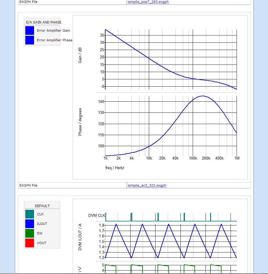
After running the test, the test report shows a fourth curve on the default graph ( scroll down to see this ). As expected the curve has the same amplitude and frequency as the VOUT curve, only the vertical axis has a different scale and is centered on zero.
This is just one example of the utility of the ArbitraryCurve function. Another application is the generation of X-Y plots. The testplan syntax documentation includes an example where the forward current and forward voltage of a diode are plotted against each other. Follow this link to the testplan syntax for more information.
6.5.2 ArbitraryBodePlot function
The ArbitraryBodePlot function plots the ratio of two complex voltages and can be used to plot the gain and phase curves of the complete feedback loop or the gain and phase of various portions of the loop, such as the error amplifier. The equivalent schematic probe symbol is the Bode Plot Probe, which can be placed from the parts selector category Probes|Bode Plot Probe - w/ Measurements. While the functionality is similar, this testplan function has a number of formatting options which increase it's flexibility. As we will see, one important such feature is the ability to probe between schematic hierarchical levels.
To demonstrate this function, let's plot the gain and phase of the compensation error amplifier in the LTC3406B circuit. This would be difficult with the schematic based probe because the output of the error amplifier is not brought out to the top level of the IC. Therefore, to use a schematic probe would require modification of the LTC3406B symbol to bring the error amplifier output to the top level. Using the ArbitraryBodePlot function solves this problem, as we can directly probe the nets in the schematic hierarchy and generate the curves without requiring any schematic modifications.
As with the other functions in section six, the ArbitraryBodePlot function is called from a measurement column. We add a measurement column and then compose the ArbitraryBodePlot function arguments. The function has four different forms which are described in the testplan syntax, and in this example we use the last form, in which we supply the four node names directly. The arguments and a brief description of each argument is described in the following table.
| Arg# | Name | Description |
|---|---|---|
| 1 | nodeIN+ | The positive input node |
| 2 | nodeIN- | The negative input node |
| 3 | nodeOUT- | The positive output node |
| 4 | nodeOUT- | The negative output node |
| 5 | curvename | The names for the curve |
| 6 | graphname | The name of the graph as seen on test report |
| 7 | gridindex | Identifies the Grid on which to place the curve |
| 8 | axisname | Identifies the Axis on a particular grid |
All measurement curve functions also take an optional final argument, OPTIONAL_PARAMETER_STRING. As the name suggests, this argument is a string containing optional curve formatting parameters. In this example, we use the OPTIONAL_PARAMETER_STRING to format our curves.
The ArbitraryBodePlot curve function has differential voltage inputs - in our case, the negative nodes are the global ground node, that is, node 0. The positive input nodes can be found from the pinnames on the symbols. First, the positive input to the probe is the SENSE pin on the load I1. Since the load is is a top level symbol, the net attached to the pinname can easily be found by concatenating the reference designator with the pinname, separated by a ".#". In our circuit, the net is I1.#SENSE.
To find the net name for the output of the error amplifier, start by opening the schematic from section 6.5.1.
LTC3406B/Test Ckts/6.5.1_LTC3406B - DVM ADVANCED.sxsch
Next, descend into U1, the top level of the LTC3406B. Then, descend into the error amplifier with reference designator U3. If the mouse cursor is moved near the output of the error amplifier, the net name and hierarchical path is shown on the bottom portion the window. In the following image, this has been highlighted with a red box. To form the complete net name, the hierarchical path and the net name will be concatenated with a "." to yield a net name of U1.U3.#OUT.
There is also a convenient keyboard shortcut which will show the net name nearest to the mouse cursor in the SIMetrix/SIMPLIS Command Shell. This keyboard shortcut is Ctrl+S, and when executed on the schematic show above, the net name is displayed in the command shell.
Net name at cursor is U1.U3.#OUT
The beginning of our ArbitraryBodePlot function showing just the first four arguments is:
ArbitraryBodePlot( I1.#SENSE , 0 , U1.U3.#OUT , 0 ,
The next argument is the curvename. The ArbitraryBodePlot function, appends the curvename provided in this argument with either the string Gain or Phase to generate unique names for the gain and phase curves. We name our curve
DVM Error Amplifier
which will generate two curves with names DVM Error Amplifier Gain and DVM Error Amplifier Phase.
The argument after the curvename is the graphname. This is the name shown in the graph legend box on the individual test reports. Let's use
E/A Gain and Phase
The final two arguments specify the gridindex and axisname. In this example, we are generating two curves and we will set the curve locations using the OPTIONAL_PARAMETER_STRING, so these two arguments are not used. There are forms of the ArbitraryBodePlot function which generate one curve, these forms require both of these arguments. Since we don't need these two arguments, we'll enter ignoreme for both arguments.
The last, and optional argument is the OPTIONAL_PARAMETER_STRING. There are many different format options, all of which are well documented in the testplan syntax. Here we will use curve=splitgain, which places the curves on two grids with the gain on the upper grid and color=blue option which will force both curves to be colored blue. The format of the final argument is:
curve=splitgain color=blue
Notice there are no commas between curve=splitgain and color=blue. This is the general format of the OPTIONAL_PARAMETER_STRING, the program is expecting a space separated string of individual options. Our complete ArbitraryBodePlot function is:
ArbitraryBodePlot( I1.#SENSE, 0, U1.U3.#OUT, 0, DVM Error Amplifier , E/A Gain and Phase , ignoreme , ignoreme , curve=splitphase color=blue )
We'll put this function into a testplan with a single test. Here we have added a single measurement column and in that column put our ArbitraryBodePlot function, both are highlighted in red.
| *** | |||||
|---|---|---|---|---|---|
| *** 6.5.2_arbitrarybodeplot.testplan arbitrarybodeplot testplan for DC/DC tutorial section 6.5.2 | |||||
| *** | |||||
| *?@ analysis | objective | measurement | source | load | label |
| *** | |||||
| Ac | BodePlot(OUTPUT:1) | ArbitraryBodePlot( I1.#SENSE , 0 , U1.U3.#OUT , 0 , DVM Error Amplifier , E/A Gain and Phase , ignoreme , ignoreme , curve=splitgain color=blue ) | SOURCE(INPUT:1, Maximum) | LOAD(OUTPUT:1, 100%) | Ac Analysis|Bode Plot|Vin Maximum|100% Load |
We are now ready to run this testplan on a LTC3406B schematic. Let's use the schematic from section 6.5.1.
LTC3406B/Test Ckts/6.5.1_LTC3406B - DVM ADVANCED.sxsch
In the test report we see our curves for the error amplifier gain and phase are formatted as expected. The curve=splitphase option has created two grids, and placed the gain curve on the upper grid. The color=blue option has formatted both curves with blue color.
A few comments may be in order. The ArbitraryBodePlot function requires a large number of arguments, which is in proportion to the power of the function. We recognized early on this may make composing the function on a reasonable sized monitor difficult. For this reason, we have also implemented the ArbitraryBodePlot function as a SIMetrix script function, to be called from a post-process script. The script based function behaves almost exactly as the testplan version, except it doesn't keep the simulation vectors. Further details are in the SIMetrix script function documentation. Using post-process scripts is discussed in section 7.2 Post-Process Scripts.
6.6 Comparing data from previous simulations
Often the entire purpose of a testplan or design of experiments is to compare the data between each test or sets of tests. To accomplish this, DVM offers two very powerful curve functions to compare simulation data in a graphical form.
The first curve function is ExtractCurve, and as it's name suggests, this function goes back to a previously run test report, opens a graph from that report, and copies the specified curve to a graph in the current test. Any number of ExtractCurve entries may be made in the testplan, allowing the comparison of curve data from multiple tests.
The second curve function, called CreateXYScalarPlot, generates a curve from the scalar data of all tests executed previous to the current test. This function was used to create the efficiency curves shown in section 5.1 Efficiency from efficiency scalar values measured in each test.
6.6.1 ExtractCurve function
The ExtractCurve function copies a curve from a previous report onto a graph in the current test report. To accomplish this, ExtractCurve looks up the previously run test by the entire test label, and then starts searching for the exact curvename in that report. If a matching curvename is found, the curve is copied to the specified graph in the current report. If no curvename match is found, a warning message is displayed in the SIMetrix/SIMPLIS command shell.
In section 6.4.3 we used the PromoteGraph and PromoteScalar functions to place graphs and scalars on the overview report. The overview scalar values for Gain Margin and Phase Margin could easily be compared in the CALCULATED RESULTS section, but the curves, being on two different graphs, were harder to compare. Let's revisit the testplan from that section and copy the curves onto a new graph, promoting this graph to the overview report. In the testplan below, we've added a measurement column (we now have five in total), and removed the PromoteGraph functions. We have also added a new test with the label "Extract Curves from Previous Reports". In the Analysis column for this test, we entered "NoSimulation", and when this test executes, the simulation is skipped and the measurement post-processing will execute and create our summary curves.
| *** | ||||||||||
|---|---|---|---|---|---|---|---|---|---|---|
| *** 6.6.1_extractcurve_start.testplan: extractcurve testplan for DC/DC tutorial section 6.6.1 | ||||||||||
| *** | ||||||||||
| *?@ analysis | objective | jumper | measurement | measurement | measurement | measurement | measurement | source | load | label |
| *** | ||||||||||
| Ac | BodePlot(OUTPUT:1) | close( J1 ) | SOURCE(INPUT:1, Nominal) | LOAD(OUTPUT:1, Light) | VOUT=1.505V|Bode Plot|Vin Nominal|Light Load | |||||
| Ac | BodePlot(OUTPUT:1) | close( J1 ) | PromoteScalar( gain_margin , Gain Margin @ 1.505V (dB)) | PromoteScalar( phase_margin , Phase Margin @ 1.505V (deg)) | SOURCE(INPUT:1, Nominal) | LOAD(OUTPUT:1, 50%) | VOUT=1.505V|Bode Plot|Vin Nominal|50% Load | |||
| Ac | BodePlot(OUTPUT:1) | close( J1 ) | SOURCE(INPUT:1, Nominal) | LOAD(OUTPUT:1, 100%) | VOUT=1.505V|Bode Plot|Vin Nominal|100% Load | |||||
| *** | ||||||||||
| *** | ||||||||||
| *** | ||||||||||
| Ac | BodePlot(OUTPUT:1) | open( J1 ) | SOURCE(INPUT:1, Nominal) | LOAD(OUTPUT:1, Light) | VOUT=0.6V|Bode Plot|Vin Nominal|Light Load | |||||
| Ac | BodePlot(OUTPUT:1) | open( J1 ) | PromoteScalar( gain_margin , Gain Margin @ 600mV (dB)) | PromoteScalar( phase_margin , Phase Margin @ 600mV (deg)) | SOURCE(INPUT:1, Nominal) | LOAD(OUTPUT:1, 50%) | VOUT=0.6V|Bode Plot|Vin Nominal|50% Load | |||
| Ac | BodePlot(OUTPUT:1) | open( J1 ) | SOURCE(INPUT:1, Nominal) | LOAD(OUTPUT:1, 100%) | VOUT=0.6V|Bode Plot|Vin Nominal|100% Load | |||||
| *** | ||||||||||
| NoSimulation | Extract Curves from Previous Reports | |||||||||
Now, we'll compose four ExtractCurve functions, two for the nominal test and two for the 600mV output voltage tests. We need two ExtractCurve functions for each test because we would like to extract the Gain and Phase curves, and the ExtractCurve function only copies a single curve. After we finish composing these, we'll add these four functions to the Extract Curves from Previous Reports test. The ExtractCurve function has six arguments, as shown in this table:
| Arg# | Name | Description |
|---|---|---|
| 1 | label | The previously run test report label |
| 2 | curvename | The name of the curve to extract |
| 3 | new curvename | The new curvename for the curve |
| 4 | graphname | The name of the graph as seen on test report |
| 5 | gridindex | Identifies the Grid which to place the curve on |
| 6 | axisname | Identifies the Axis on a particular grid |
ExtractCurve function for the Phase curve generated by the nominal output voltage test. The label for this test is:
VOUT=1.505V|Bode Plot|Vin Nominal|50% Load
and the curvename to be extracted is:
DVM Phase
So we can differentiate between our two sets of curves, we want to rename the curve when we extract it to the new graph. Our new curvename needs to describe the test conditions and is:
DVM Phase @ 1.505V
Now we need to choose a graph name.
Bode Plot Summary
should work quite well. This will be the graphname displayed on the overview report.
Finally, the gridindex - in this example, we'll place the gain curve on a new grid above the phase curve, so we will choose A1, which represents the first (lowest) analog grid. As we will see, the Gain curve will have a gridindex of A2, representing the second analog grid. The axisname isn't important as we are only planning to have a single axis on the lower grid. We'll use bodemag for the Gain curves and bodephase for the Phase curves, as these are the names used by a fixed schematic probe.
As with the other curve functions, there is an OPTIONAL_PARAMETER_STRING for the last argument. We need to at least put a option for setting the x axis to log scale, as the ExtractCurve function doesn't copy this from the original graph. We also want our curves to have the same color - this makes it easier to determine which curve belongs to which set of data. So, we'll set our OPTIONAL_PARAMETER_STRING to:
xScale=log color=red
We can now compose the entire function. Our ExtractCurve Phase function should be:
| ExtractCurve( VOUT=1.505V|Bode Plot|Vin Nominal|50% Load , DVM Phase , DVM Phase @ 1.505V , Bode Plot Summary , A1 , bodephase , xScale=log color=red ) |
We now have one curve function completed. Before you feel totally overwhelmed, we are actually most of the way to having all four curve functions complete. To create our Gain function, all we need to do is copy the Phase function and make a few small changes:
- Replace all
Phaseentries withGain - Change the gridindex from
A1toA2 - Change the axisname from
bodephasetobodemag
ExtractCurve functions for nominal output voltage test will be:
| ExtractCurve( VOUT=1.505V|Bode Plot|Vin Nominal|50% Load , DVM Phase , DVM Phase @ 1.505V , Bode Plot Summary , A1 , bodephase , xScale=log color=red ) |
| ExtractCurve( VOUT=1.505V|Bode Plot|Vin Nominal|50% Load , DVM Gain , DVM Gain @ 1.505V , Bode Plot Summary , A2 , bodemag , xScale=log color=red ) |
At this point we have composed the ExtractCurve functions for the first test, and we can easily duplicate both functions, making the following changes:
- Change the label from
VOUT=1.505V|Bode Plot|Vin Nominal|50% LoadtoVOUT=0.6V|Bode Plot|Vin Nominal|50% Load - Change the curvenames, replacing the
1.505Vwith600mV - Change the color from
redto another color, sayblue
Our final four ExtractCurve functions, with the changes in red, will be:
| ExtractCurve( VOUT=1.505V|Bode Plot|Vin Nominal|50% Load , DVM Phase , DVM Phase @ 1.505V , Bode Plot Summary , A1 , bodephase , xScale=log color=red ) |
| ExtractCurve( VOUT=1.505V|Bode Plot|Vin Nominal|50% Load , DVM Gain , DVM Gain @ 1.505V , Bode Plot Summary , A2 , bodemag , xScale=log color=red ) |
| ExtractCurve( VOUT=0.6V|Bode Plot|Vin Nominal|50% Load , DVM Phase , DVM Phase @ 600mV , Bode Plot Summary , A1 , bodephase , xScale=log color=blue ) |
| ExtractCurve( VOUT=0.6V|Bode Plot|Vin Nominal|50% Load , DVM Gain , DVM Gain @ 600mV , Bode Plot Summary , A2 , bodemag , xScale=log color=blue ) |
PromoteGraph entry to place the summary curves on the overview report, our finished testplan will look like the following.
| *** | ||||||||||
|---|---|---|---|---|---|---|---|---|---|---|
| *** 6.6.1_extractcurve_final.testplan: extractcurve testplan for DC/DC tutorial section 6.6.1 | ||||||||||
| *** | ||||||||||
| *?@ analysis | objective | jumper | measurement | measurement | measurement | measurement | measurement | source | load | label |
| *** | ||||||||||
| Ac | BodePlot(OUTPUT:1) | close( J1 ) | SOURCE(INPUT:1, Nominal) | LOAD(OUTPUT:1, Light) | VOUT=1.505V|Bode Plot|Vin Nominal|Light Load | |||||
| Ac | BodePlot(OUTPUT:1) | close( J1 ) | PromoteScalar( gain_margin , Gain Margin @ 1.505V (dB)) | PromoteScalar( phase_margin , Phase Margin @ 1.505V (deg)) | SOURCE(INPUT:1, Nominal) | LOAD(OUTPUT:1, 50%) | VOUT=1.505V|Bode Plot|Vin Nominal|50% Load | |||
| Ac | BodePlot(OUTPUT:1) | close( J1 ) | SOURCE(INPUT:1, Nominal) | LOAD(OUTPUT:1, 100%) | VOUT=1.505V|Bode Plot|Vin Nominal|100% Load | |||||
| *** | ||||||||||
| *** | ||||||||||
| *** | ||||||||||
| Ac | BodePlot(OUTPUT:1) | open( J1 ) | SOURCE(INPUT:1, Nominal) | LOAD(OUTPUT:1, Light) | VOUT=0.6V|Bode Plot|Vin Nominal|Light Load | |||||
| Ac | BodePlot(OUTPUT:1) | open( J1 ) | PromoteScalar( gain_margin , Gain Margin @ 600mV (dB)) | PromoteScalar( phase_margin , Phase Margin @ 600mV (deg)) | SOURCE(INPUT:1, Nominal) | LOAD(OUTPUT:1, 50%) | VOUT=0.6V|Bode Plot|Vin Nominal|50% Load | |||
| Ac | BodePlot(OUTPUT:1) | open( J1 ) | SOURCE(INPUT:1, Nominal) | LOAD(OUTPUT:1, 100%) | VOUT=0.6V|Bode Plot|Vin Nominal|100% Load | |||||
| *** | ||||||||||
| NoSimulation | ExtractCurve( VOUT=1.505V|Bode Plot|Vin Nominal|50% Load , DVM Phase , DVM Phase @ 1.505V , Bode Plot Summary , A1 , bodephase , xScale=log color=red ) | ExtractCurve( VOUT=1.505V|Bode Plot|Vin Nominal|50% Load , DVM Gain , DVM Gain @ 1.505V , Bode Plot Summary , A2 , bodemag , xScale=log color=red ) | ExtractCurve( VOUT=0.6V|Bode Plot|Vin Nominal|50% Load , DVM Phase , DVM Phase @ 600mV , Bode Plot Summary , A1 , bodephase , xScale=log color=blue ) | ExtractCurve( VOUT=0.6V|Bode Plot|Vin Nominal|50% Load , DVM Gain , DVM Gain @ 600mV , Bode Plot Summary , A2 , bodemag , xScale=log color=blue ) | PromoteGraph( Bode Plot Summary ) | Extract Curves from Previous Reports | ||||
A copy of this testplan can be found in the download directory:
testplans/6.6.1_extractcurve_final.testplan
We can now run this testplan on the schematic from section 6.3:
LTC3406B/Test Ckts/6.3_LTC3406B - DVM ADVANCED.sxsch
As expected, the overview report contains the BODE PLOT SUMMARY graph summarizing the Bode Plots with four curves. The four measured scalar values for Gain and Phase Margin are shown in the CALCULATED RESULTS section.
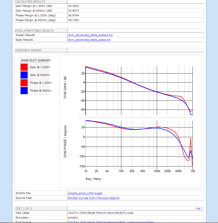
A few notes about possible warnings displayed in the SIMetrix/SIMPLIS command shell. After tests are selected to be run, but before the testplan is executed, DVM will audit the testplan for syntax and for any tests not selected, but are required by later tests. For example, if the same testplan was run, but only the test with label:
VOUT=1.505V|Bode Plot|Vin Nominal|50% Load
and the summary test were selected, the following errors would be displayed in the SIMetrix/SIMPLIS command shell:
Test #2 attempts to extract a curve from a test with the label VOUT=0.6V|Bode Plot|Vin Nominal|50% Load which is not selected to have been run before Test #2 is set to be executed.

Test #2 attempts to extract a curve from a test with the label VOUT=0.6V|Bode Plot|Vin Nominal|50% Load which is not selected to have been run before Test #2 is set to be executed.
These two warnings, one for each ExtractCurve function, simply warn you the final graph might not have all the curves which you might expect to find if the entire testplan was run.
Common with the other curve functions, the ExtractCurve function requires a large number of arguments. We recognized early on this may make composing the function on a reasonable sized monitor difficult. For this reason, we have also implemented the ExtractCurve function as a SIMetrix script function, to be called from a post-process script. The script based function behaves exactly as the testplan version. The syntax for this function is described in the SIMetrix script function documentation. Using post-process scripts is discussed in section 7.2 Post-Process Scripts.
6.6.2 CreateXYScalarPlot function
In section 5.1 Efficiency, we simulated the efficiency of the converter using the built-in Efficiency testplan. The final graph produced in that section plotted three efficiency curves taken from scalar data aggregated from the previous tests. Three CreateXYScalarPlot functions were used to generate these curves. A copy of the efficiency testplan is included in the download directory:
testplans/dvm_builtin-efficiency_dcdc_1in_1out.testplan
The CreateXYScalarPlot requires seven arguments with an optional eighth, the OPTIONAL_PARAMETER_STRING.
| Arg# | Name | Description |
|---|---|---|
| 1 | x-expression | The expression of scalars to be plotted on the x-axis |
| 2 | y-expression | The expression of scalars to be plotted on the y-axis |
| 3 | scalars to extract | A space delimited list of scalars to extract from the previous reports. |
| 4 | curvename | Name for the curve being generated |
| 5 | graphname | The name of the graph as seen on test report |
| 6 | gridindex | Identifies the Grid which to place the curve on |
| 7 | axisname | Identifies the Axis on a particular grid |
In the simplest case, the scalar expressions x-expression and y-expression can be any scalars from the test reports. In more complex applications, the expressions can be any mathematical expression of scalar values, values set with the Var, Globalvar, Change testplan entries. In the built-in efficiency testplan, we plot the efficiency vs. the load current, both of which are single scalar values. The x-expression is
AVG(ILOAD)
and the y-expression is
Efficiency_Nom
which is a scalar alias created with the Alias function.
The third argument is the list of scalars to extract from the previous reports. This argument is composed of a space delimited list of scalar values used in the x-expression and y-expression. DVM automatically makes the variable defined with Var, Globalvar and Change testplan entries available. For this reason, these "scalars" should not be included in this list. Our third argument is therefore:
AVG(ILOAD) Efficiency_Nom
The curvename should be prefixed with DVM in order for DVM to retain the curve on the overview and test report graphs. In our case, we choose:
DVM Vin Nom
for the nominal input voltage case.
The graphname is next, and since we are plotting various efficiency curves, we choose
DVM Efficiency
The sixth and seventh arguments are the gridindex and axisname. Since we only have one graph, with three curves, we will use gridindex
A1
the default grid. And since we don't have multiple axes, the axisname isn't important, and we will use
vert
The optional eighth argument OPTIONAL_PARAMETER_STRING will almost always be used with the CreateXYScalarPlot function, as the resulting graph will need annotation. Using this argument, we can set almost every important graph annotation, from labels, units, even major grid spacing.
We need to set the axis labels , axis units, curve color and in this case, we desire to see the actual data points. The following string will set all of these properties:
xlabel=Load Current xunits=A ylabel=Efficiency yunits=%%% showpoints=true color=red
The full range of options is described in the testplan syntax documentation.
We now have the complete CreateXYScalarPlot function for the nominal input voltage
| CreateXYScalarPlot( AVG(ILOAD) , Efficiency_Nom , AVG(ILOAD) Efficiency_Nom , DVM Vin Nom , DVM Efficiency , A1, vert, xlabel=Load Current xunits=A ylabel=Efficiency yunits=%%% showpoints=true color=red) |
Now that we have composed the Nominal input voltage CreateXYScalarPlot function, we can copy it and easily build the other two functions for the Minimum and Maximum input voltage. After duplicating the existing function twice, we need to change only two items:
- Replace all
Nomentries withMinand thenMax - Change the curve colors to green and blue
The final three functions are shown below.
| CreateXYScalarPlot( AVG(ILOAD) , Efficiency_Nom , AVG(ILOAD) Efficiency_Nom , DVM Vin Nom , DVM Efficiency , A1, vert, xlabel=Load Current xunits=A ylabel=Efficiency yunits=%%% showpoints=true color=red) |
| CreateXYScalarPlot( AVG(ILOAD) , Efficiency_Min , AVG(ILOAD) Efficiency_Min , DVM Vin Min , DVM Efficiency , A1, vert, xlabel=Load Current xunits=A ylabel=Efficiency yunits=%%% showpoints=true color=green) |
| CreateXYScalarPlot( AVG(ILOAD) , Efficiency_Max , AVG(ILOAD) Efficiency_Max , DVM Vin Max , DVM Efficiency , A1, vert, xlabel=Load Current xunits=A ylabel=Efficiency yunits=%%% showpoints=true color=blue) |
After these three CreateXYScalarPlot measurements are entered into the testplan, we have the built-in testplan from section 5.1.
| *** | ||||||||
|---|---|---|---|---|---|---|---|---|
| *** efficiency_dcdc_1in_1out.testplan | ||||||||
| *** | ||||||||
| *?@ analysis | objective | source | load | label | Measurement | Measurement | Measurement | Measurement |
| *** | ||||||||
| *** | ||||||||
| Steady-State | Steady-State | SOURCE(INPUT:1, Nominal) | LOAD(OUTPUT:1, Light) | Steady-State|Steady-State|Vin Nominal|Light Load | Alias( Efficiency, Efficiency_nom) | |||
| Steady-State | Steady-State | SOURCE(INPUT:1, Nominal) | LOAD(OUTPUT:1, 10%) | Steady-State|Steady-State|Vin Nominal|10% | Alias( Efficiency, Efficiency_nom) | |||
| Steady-State | Steady-State | SOURCE(INPUT:1, Nominal) | LOAD(OUTPUT:1, 20%) | Steady-State|Steady-State|Vin Nominal|20% | Alias( Efficiency, Efficiency_nom) | |||
| Steady-State | Steady-State | SOURCE(INPUT:1, Nominal) | LOAD(OUTPUT:1, 30%) | Steady-State|Steady-State|Vin Nominal|30% | Alias( Efficiency, Efficiency_nom) | |||
| Steady-State | Steady-State | SOURCE(INPUT:1, Nominal) | LOAD(OUTPUT:1, 40%) | Steady-State|Steady-State|Vin Nominal|40% | Alias( Efficiency, Efficiency_nom) | |||
| Steady-State | Steady-State | SOURCE(INPUT:1, Nominal) | LOAD(OUTPUT:1, 50%) | Steady-State|Steady-State|Vin Nominal|50% | Alias( Efficiency, Efficiency_nom) | |||
| Steady-State | Steady-State | SOURCE(INPUT:1, Nominal) | LOAD(OUTPUT:1, 60%) | Steady-State|Steady-State|Vin Nominal|60% | Alias( Efficiency, Efficiency_nom) | |||
| Steady-State | Steady-State | SOURCE(INPUT:1, Nominal) | LOAD(OUTPUT:1, 70%) | Steady-State|Steady-State|Vin Nominal|70% | Alias( Efficiency, Efficiency_nom) | |||
| Steady-State | Steady-State | SOURCE(INPUT:1, Nominal) | LOAD(OUTPUT:1, 80%) | Steady-State|Steady-State|Vin Nominal|80% | Alias( Efficiency, Efficiency_nom) | |||
| Steady-State | Steady-State | SOURCE(INPUT:1, Nominal) | LOAD(OUTPUT:1, 90%) | Steady-State|Steady-State|Vin Nominal|90% | Alias( Efficiency, Efficiency_nom) | |||
| Steady-State | Steady-State | SOURCE(INPUT:1, Nominal) | LOAD(OUTPUT:1, 100%) | Steady-State|Steady-State|Vin Nominal|100% | Alias( Efficiency, Efficiency_nom) | |||
| *** | ||||||||
| Steady-State | Steady-State | SOURCE(INPUT:1, Maximum) | LOAD(OUTPUT:1, Light) | Steady-State|Steady-State|Vin Maximum|Light Load | Alias( Efficiency, Efficiency_Max) | |||
| Steady-State | Steady-State | SOURCE(INPUT:1, Maximum) | LOAD(OUTPUT:1, 10%) | Steady-State|Steady-State|Vin Maximum|10% | Alias( Efficiency, Efficiency_Max) | |||
| Steady-State | Steady-State | SOURCE(INPUT:1, Maximum) | LOAD(OUTPUT:1, 20%) | Steady-State|Steady-State|Vin Maximum|20% | Alias( Efficiency, Efficiency_Max) | |||
| Steady-State | Steady-State | SOURCE(INPUT:1, Maximum) | LOAD(OUTPUT:1, 30%) | Steady-State|Steady-State|Vin Maximum|30% | Alias( Efficiency, Efficiency_Max) | |||
| Steady-State | Steady-State | SOURCE(INPUT:1, Maximum) | LOAD(OUTPUT:1, 40%) | Steady-State|Steady-State|Vin Maximum|40% | Alias( Efficiency, Efficiency_Max) | |||
| Steady-State | Steady-State | SOURCE(INPUT:1, Maximum) | LOAD(OUTPUT:1, 50%) | Steady-State|Steady-State|Vin Maximum|50% | Alias( Efficiency, Efficiency_Max) | |||
| Steady-State | Steady-State | SOURCE(INPUT:1, Maximum) | LOAD(OUTPUT:1, 60%) | Steady-State|Steady-State|Vin Maximum|60% | Alias( Efficiency, Efficiency_Max) | |||
| Steady-State | Steady-State | SOURCE(INPUT:1, Maximum) | LOAD(OUTPUT:1, 70%) | Steady-State|Steady-State|Vin Maximum|70% | Alias( Efficiency, Efficiency_Max) | |||
| Steady-State | Steady-State | SOURCE(INPUT:1, Maximum) | LOAD(OUTPUT:1, 80%) | Steady-State|Steady-State|Vin Maximum|80% | Alias( Efficiency, Efficiency_Max) | |||
| Steady-State | Steady-State | SOURCE(INPUT:1, Maximum) | LOAD(OUTPUT:1, 90%) | Steady-State|Steady-State|Vin Maximum|90% | Alias( Efficiency, Efficiency_Max) | |||
| Steady-State | Steady-State | SOURCE(INPUT:1, Maximum) | LOAD(OUTPUT:1, 100%) | Steady-State|Steady-State|Vin Maximum|100% | Alias( Efficiency, Efficiency_Max) | |||
| *** | ||||||||
| Steady-State | Steady-State | SOURCE(INPUT:1, Minimum) | LOAD(OUTPUT:1, Light) | Steady-State|Steady-State|Vin Minimum|Light Load | Alias( Efficiency, Efficiency_Min) | |||
| Steady-State | Steady-State | SOURCE(INPUT:1, Minimum) | LOAD(OUTPUT:1, 10%) | Steady-State|Steady-State|Vin Minimum|10% | Alias( Efficiency, Efficiency_Min) | |||
| Steady-State | Steady-State | SOURCE(INPUT:1, Minimum) | LOAD(OUTPUT:1, 20%) | Steady-State|Steady-State|Vin Minimum|20% | Alias( Efficiency, Efficiency_Min) | |||
| Steady-State | Steady-State | SOURCE(INPUT:1, Minimum) | LOAD(OUTPUT:1, 30%) | Steady-State|Steady-State|Vin Minimum|30% | Alias( Efficiency, Efficiency_Min) | |||
| Steady-State | Steady-State | SOURCE(INPUT:1, Minimum) | LOAD(OUTPUT:1, 40%) | Steady-State|Steady-State|Vin Minimum|40% | Alias( Efficiency, Efficiency_Min) | |||
| Steady-State | Steady-State | SOURCE(INPUT:1, Minimum) | LOAD(OUTPUT:1, 50%) | Steady-State|Steady-State|Vin Minimum|50% | Alias( Efficiency, Efficiency_Min) | |||
| Steady-State | Steady-State | SOURCE(INPUT:1, Minimum) | LOAD(OUTPUT:1, 60%) | Steady-State|Steady-State|Vin Minimum|60% | Alias( Efficiency, Efficiency_Min) | |||
| Steady-State | Steady-State | SOURCE(INPUT:1, Minimum) | LOAD(OUTPUT:1, 70%) | Steady-State|Steady-State|Vin Minimum|70% | Alias( Efficiency, Efficiency_Min) | |||
| Steady-State | Steady-State | SOURCE(INPUT:1, Minimum) | LOAD(OUTPUT:1, 80%) | Steady-State|Steady-State|Vin Minimum|80% | Alias( Efficiency, Efficiency_Min) | |||
| Steady-State | Steady-State | SOURCE(INPUT:1, Minimum) | LOAD(OUTPUT:1, 90%) | Steady-State|Steady-State|Vin Minimum|90% | Alias( Efficiency, Efficiency_Min) | |||
| Steady-State | Steady-State | SOURCE(INPUT:1, Minimum) | LOAD(OUTPUT:1, 100%) | Steady-State|Steady-State|Vin Minimum|100% | Alias( Efficiency, Efficiency_Min) | |||
| *** | ||||||||
| NoSimulation | Steady-State|Generate Efficiency Curves | CreateXYScalarPlot( AVG(ILOAD) , Efficiency_Min , AVG(ILOAD) Efficiency_Min , DVM Vin Min , DVM Efficiency , A1, vert, xlabel=Load Current xunits=A ylabel=Efficiency yunits=%%% showpoints=true color=green) | CreateXYScalarPlot( AVG(ILOAD) , Efficiency_Nom , AVG(ILOAD) Efficiency_Nom , DVM Vin Nom , DVM Efficiency , A1, vert, xlabel=Load Current xunits=A ylabel=Efficiency yunits=%%% showpoints=true color=red) | CreateXYScalarPlot( AVG(ILOAD) , Efficiency_Max , AVG(ILOAD) Efficiency_Max , DVM Vin Max , DVM Efficiency , A1, vert, xlabel=Load Current xunits=A ylabel=Efficiency yunits=%%% showpoints=true color=blue) | PromoteGraph( DVM Efficiency , 1 ) | |||
7.0 Miscellaneous Topics
SIMetrix/SIMPLIS ships with a powerful scripting language (script documentation). DVM allows for users to specify pre- and post-processing scripts to be run with a test. Pre- and post-processing scripts can be assigned either in a testplan (testplan syntax documentation) or through the DVM Control (supported by both the Basic and Full PowerAssist symbols). Scripts called from the testplan can be assigned on a test-by-test basis, while scripts assigned in the DVM Control Symbol will be called during every test. Pre- and post-process scripts are launched with the /quiet and /noerr flags to prevent script errors from halting DVM execution.
A note about debugging pre- and post-process scripts. Because the scripts are executed with the /noerr and /quiet flags, error generation is suppressed. This makes debugging scripts difficult and therefore an unsupported option has been included to execute the scripts without these flags. The option is named "SimplisDVMPostProcessDebug" and can be turned on by copying and pasting the following into the SIMetrix/SIMPLIS Command Line:
Set SimplisDVMPostProcessDebug
Once the script has been debugged, the option can be removed by issuing the command:
Unset SimplisDVMPostProcessDebug
A standard interface for both pre-process and post-process scripts has been developed. This standard interface is set with the following Arguments definition in the script file. You can copy this line and paste it into each script file you use, both pre- and post-process.
Arguments @retval label report_dir log_file controlhandle
retval is the return value for the script. For preprocess scripts, the return value is logged in the test log file, while for post-process scripts, the scalars are returned on the first index (retval[0]), and specifications are returned on the second index (retval[1]). Details are described in section 7.3 User-Defined Scalar and Spec Values.
label is the label of the currently executing test. Since the label is passed to both the pre-process and post-process scripts, the script can decode the label and determine which test is currently executing. This allows the script to modify values or make measurements based on the currently executing test.
report_dir is the base directory for simulation results.
log_file is the location of the overview log.
controlhandle is the value of the Handle property for the DVM Control Symbol on the top level schematic. The script function PropValues2() can read values from the DVM control symbol using the controlhandle value.
Multiple Pre- and post-scripts can be assigned using the testplan headers preprocess, postprocess and finalprocess. If multiple scripts are assigned, the order of their execution is as follows:
- scripts assigned in the testplan, from left to right within the test definition row
- scripts assigned in the control symbol
7.1 Pre-Process Scripts
Pre-process scripts are executed immediately before the simulation is launched. At this point, the simulation analysis has already been set in the F11 window of the schematic. This order of operations allows a user to override any automatic DVM action with a pre-process script.
7.2 Post-Process and Final-Process Scripts
Post-process scripts are executed after the simulation is completed and before any waveform processing is started. Final-Process scripts are executed after DVM processes the waveforms, and in some test modes, DVM will actually create new curves. If measurements on those curves are to be made, make certain your script is called from a finalprocess testplan column.
7.3 User-Defined Scalar and Spec Values
The retval string vector is used to return both scalar and specification values from post-process and final-process scripts. In the case of pre-process scripts, there are no scalar values to return, however, the returned value, retval is written to the Log File. This allows a pass/fail status message to be passed to the Log File from the pre-process script. For example, a preprocess script which successfully executed might return to following, with strings colored green and commands red.
Let retval = 'preprocess script executed properly'
SimplisDVMAdvancedUtilCreateScalar function. The function takes two arguments, with an optional third argument. All arguments are strings - this means you should change your calculated scalar value to a string using the Str() or FormatNumber() SIMetrix script function. The two forms for the SimplisDVMAdvancedUtilCreateScalar function are:
SimplisDVMAdvancedUtilCreateScalar( scalarname , scalarvalue )SimplisDVMAdvancedUtilCreateScalar( scalarname , scalarvalue , existing scalarnames )
scalarname is any string, not containing spaces, equal signs, or the tilde "~" character. The scalarvalue is expected to be a string representation of the scalar's value. As an example, the following two command sequence will return a single scalar with name my_pi with value 3.1415927, note the value 3.1415927 is enclosed in single quotes, denoting a string.:
Let user_scalars = SimplisDVMAdvancedUtilCreateScalar( 'my_pi' , '3.1415927' )Let retval = [ user_scalars ]
To return multiple scalar values, we pass the existing scalars as the third argument to the function:
Let user_scalars = SimplisDVMAdvancedUtilCreateScalar( 'my_pi' , '3.1415927' )Let user_scalars = SimplisDVMAdvancedUtilCreateScalar( 'my_2pi' , '6.2831853' , user_scalars )Let retval = [ user_scalars ]
This process can be repeated for each scalar value which is returned. The final Let retval = [ user_scalars ] command will assign all the scalar values to the return value from the script. This line must come after all scalar values are assigned using the SimplisDVMAdvancedUtilCreateScalar function.
SimplisDVMAdvancedUtilCreateSpec function creates the specification value and has three required arguments with an optional fourth argument. As with the scalar function, all arguments are strings. The two forms of the SimplisDVMAdvancedUtilCreateSpec function are:
SimplisDVMAdvancedUtilCreateSpec( specname , status , description )SimplisDVMAdvancedUtilCreateSpec( specname , status , description , existing specs)
Where specname can be any string, not containing spaces, equal signs, or the tilde "~" character. The status can be either 'PASS' , 'FAIL' , or 'WARN'. Note the single quotes which, in the script language, denote these as strings. The description can be any string containing spaces, and will be displayed on the test report next to the scalar value and the pass/fail/warn status.
To create a single specification value which passes:
Let user_specs = SimplisDVMAdvancedUtilCreateSpec( 'is_value_pi', 'PASS', '3.1415927 is pi' )Let retval = [ '' , user_specs ]
to return multiple spec values, pass the existing specs as the fourth argument to the function:
Let user_specs = SimplisDVMAdvancedUtilCreateSpec( 'is_value_pi', 'PASS', '3.1415927 is pi' )Let user_specs = SimplisDVMAdvancedUtilCreateSpec( 'is_value_2pi', 'FAIL', '3.1415927 is not 2*pi' , user_specs )Let retval = [ '' , user_specs ]
In these examples, only scalars or specs were returned using the two lines:
Let retval = [ user_scalars ]Let retval = [ '' , user_specs ]
Of course, both scalars and specs can be returned by assigning both user_scalars and user_specs to the retval as follows:
Let retval = [ user_scalars , user_specs ]
A pre-prepared testplan which calls a pre and post process scripts is included in the download file:
testplans/7.3_pre_and_post_process.testplan
The testplan contains six tests, calling the preprocess in one test, and the poet process script in the other five. The testplan is shown below:
| *** | ||
|---|---|---|
| *** 7.3_pre_and_post_process.testplan: pre and post process testplan for DC/DC tutorial section 7.3 | ||
| *** | ||
| *?@ label | preprocess | postprocess |
| *** | ||
| Pre-Process | ../../scripts/7.3_pre_process.sxscr | |
| Post-Process 1 Scalar | ../../scripts/7.3_post_process.sxscr | |
| Post-Process 2 Scalars | ../../scripts/7.3_post_process.sxscr | |
| Post-Process 1 Spec | ../../scripts/7.3_post_process.sxscr | |
| Post-Process 2 Specs | ../../scripts/7.3_post_process.sxscr | |
| Post-Process w/ 2 Scalars and 2 Specs | ../../scripts/7.3_post_process.sxscr | |
This testplan calls two scripts, one in pre-process and one in post-process. Note the relative path to the scripts - up two directories to the download directory, then down one directory into the scripts directory. Both scripts are available in the download directory:
scripts/7.3_pre_process.sxscrscripts/7.3_post_process.sxscr
This testplan can be run on any of the schematics in the LTC3406B\Test Ckts directory. After running the entire testplan on the schematic
LTC3406B/Test Ckts/6.3_LTC3406B-DVM-ADVANCED.sxsch
The resulting overview report will have have six tests with tests #5 and #6 failing. These test fail because the post process script returned a specification value which was a 'FAIL'.
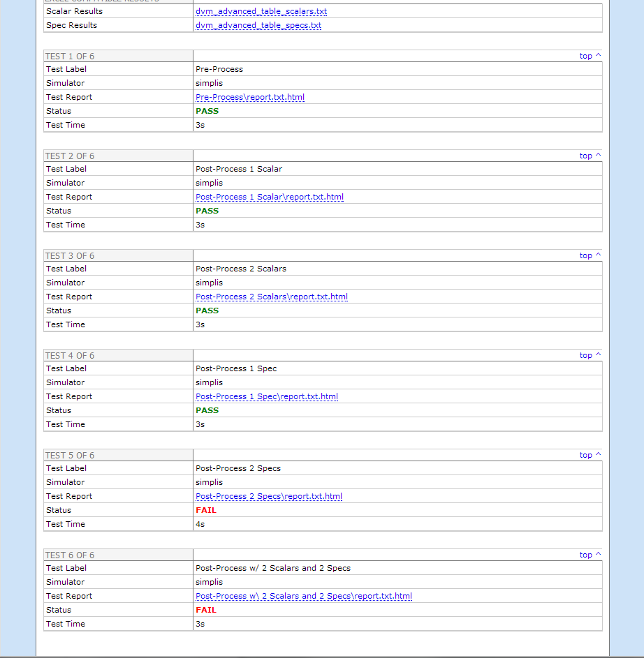
8.0 Applications
In the preceding sections, we have covered all the important DVM operations and testplan syntax. Now it's time to apply these functions to real examples, and to solve real problems. The focus in the following examples is therefore on how we apply these functions rather than on the syntax. Should any questions arise on the syntax or function being used, the preceding sections or the testplan syntax web page may be consulted. Often the testplans and scripts in these sections will be compatible with one of your circuits, without modification.
8.1 Adding Power Losses to an Efficiency Testplan
The built-in efficiency testplan measures the overall efficiency of the converter. What about adding individual power losses to the report so we can observe how the power losses vary over line and load changes? Or can we separate the gate drive power loss from the input source power of the circuit? It turns out both are easy to add to the built-in efficiency testplan. In this example, five graphs are generated, including the total losses (switching and conduction) for the MOSFETs in a Sync Buck circuit. The other three graphs include the overall efficiency, Gate Drive Power loss, and remaining losses in the circuit. To plot the remaining power losses, we will use a very powerful feature of the CreateXYScalarPlot function, that is the ability to plot mathematical expressions of measured scalar values. We will use a new example schematic which uses discrete packaged MOSFETs. This will allow the MOSFET losses to be measured directly. The efficiency and power loss schematic for our example is:
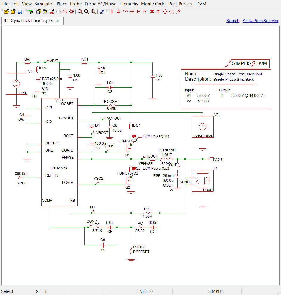
The schematic is included in the download directory at:
ISL6527A\8.1_Sync Buck Efficiency.sxsch
When compared with our previous schematics, you may notice a few things new symbols:
- Fixed power probes have been placed on the MOSFETs Q1 and Q2. These also have the "mean" fixed probe measurement applied. These probes generate the scalar values for the total loss in the devices.
- A second input source has been added to supply power to the high-side gate driver. When DVM calculates the efficiency of a circuit it includes the power from all input sources and all output loads. The individual power delivered by each input source and dissipated by each output load is also measured and reported as a scalar value.
This prepared schematic will run exactly like the built-in efficiency testplan. The scalar values will be generated by the probes and by DVM, those scalars are then assigned aliases based on the input voltage for the test. Finally, after all the tests complete, a final test is executed which generates the summary curves. Instead of using the measurement column to define our CreateXYScalarPlot curve functions, we have put these in a finalprocess script. This makes the testplan more manageable. The script is available in the download directory.
scripts/8.1_efficiency_and_powerloss_post_process.sxscr
The one portion of this script which needs discussing is the scalar expression capabilities of the CreateXYScalarPlot function. For example, one of the CreateXYScalarPlot functions is:
Let ignoreme = SimplisDVMAdvancedUtilMeasurementCreateXYScalarPlot([ 'ILOAD_Nom' , 'Power_Line_Nom - Power_Load_Nom - Power_Q1_Nom - Power_Q2_Nom + Power_Gate_Drive_Nom' , 'ILOAD_Nom Power_Line_Nom Power_Load_Nom Power_Q1_Nom Power_Q2_Nom Power_Gate_Drive_Nom' , 'DVM Vin Nom' , 'DVM Remaining Power Loss' , 'A1' , 'vert' , 'xlabel=Load Current xunits=A ylabel=Power Loss yunits=W showpoints=true color=blue' ] , log_file )
The second argument of this function is the mathematical expression of the remaining power loss once the input line, output load, gate drive, and MOSFET power losses have been removed.
'Power_Line_Nom - Power_Load_Nom - Power_Q1_Nom - Power_Q2_Nom + Power_Gate_Drive_Nom'
This is is a good example of scalar mathematics. DVM will evaluate this expression on a point by point basis and plot the resulting values.
The testplan for this schematic example is included in the tutorial download directory:
testplans/8.1_efficiency_and_powerloss.testplan
The testplan is similar to the built-in efficiency testplan we ran in section 5.1. It differs in that we now have two source columns, because we added a second input source, and additional measurement columns for the scalar aliases. Finally, on the last line of the testplan, there is a single finalprocess entry for the post processing script. This script has a path which is relative to the schematic: ..\scripts\8.1_efficiency_and_powerloss_post_process.sxscr. We have also added additional tests for the lower load currents, in order to fill in the efficiency curve points. This testplan uses 5% load steps from 5% to 40% of full load, and 10% load steps from 40% to 100% of full load.
| *** | |||||||||||||
|---|---|---|---|---|---|---|---|---|---|---|---|---|---|
| *** 8.1_efficiency_and_powerloss.testplan | |||||||||||||
| *** | |||||||||||||
| *?@ analysis | objective | source | source | load | label | Measurement | Measurement | Measurement | Measurement | Measurement | Measurement | Measurement | finalprocess |
| *** | |||||||||||||
| *** | |||||||||||||
| Steady-State | Steady-State | SOURCE(INPUT:1, Nominal) | SOURCE(INPUT:2, Nominal) | LOAD(OUTPUT:1, 5%) | Steady-State|Steady-State|Vin Nominal|5% | Alias( Efficiency, Efficiency_nom) | Alias( AVG(ILoad), ILOAD_Nom ) | Alias( AVG(Power(Q1)) , Power_Q1_Nom ) | Alias( AVG(Power(Q2)) , Power_Q2_Nom ) | Alias( Power(Line) , Power_Line_Nom ) | Alias( Power(Load) , Power_Load_Nom ) | Alias( Power(Gate_Drive) , Power_Gate_Drive_Nom ) | |
| Steady-State | Steady-State | SOURCE(INPUT:1, Nominal) | SOURCE(INPUT:2, Nominal) | LOAD(OUTPUT:1, 10%) | Steady-State|Steady-State|Vin Nominal|10% | Alias( Efficiency, Efficiency_nom) | Alias( AVG(ILoad), ILOAD_Nom ) | Alias( AVG(Power(Q1)) , Power_Q1_Nom ) | Alias( AVG(Power(Q2)) , Power_Q2_Nom ) | Alias( Power(Line) , Power_Line_Nom ) | Alias( Power(Load) , Power_Load_Nom ) | Alias( Power(Gate_Drive) , Power_Gate_Drive_Nom ) | |
| Steady-State | Steady-State | SOURCE(INPUT:1, Nominal) | SOURCE(INPUT:2, Nominal) | LOAD(OUTPUT:1, 15%) | Steady-State|Steady-State|Vin Nominal|15% | Alias( Efficiency, Efficiency_nom) | Alias( AVG(ILoad), ILOAD_Nom ) | Alias( AVG(Power(Q1)) , Power_Q1_Nom ) | Alias( AVG(Power(Q2)) , Power_Q2_Nom ) | Alias( Power(Line) , Power_Line_Nom ) | Alias( Power(Load) , Power_Load_Nom ) | Alias( Power(Gate_Drive) , Power_Gate_Drive_Nom ) | |
| Steady-State | Steady-State | SOURCE(INPUT:1, Nominal) | SOURCE(INPUT:2, Nominal) | LOAD(OUTPUT:1, 20%) | Steady-State|Steady-State|Vin Nominal|20% | Alias( Efficiency, Efficiency_nom) | Alias( AVG(ILoad), ILOAD_Nom ) | Alias( AVG(Power(Q1)) , Power_Q1_Nom ) | Alias( AVG(Power(Q2)) , Power_Q2_Nom ) | Alias( Power(Line) , Power_Line_Nom ) | Alias( Power(Load) , Power_Load_Nom ) | Alias( Power(Gate_Drive) , Power_Gate_Drive_Nom ) | |
| Steady-State | Steady-State | SOURCE(INPUT:1, Nominal) | SOURCE(INPUT:2, Nominal) | LOAD(OUTPUT:1, 25%) | Steady-State|Steady-State|Vin Nominal|25% | Alias( Efficiency, Efficiency_nom) | Alias( AVG(ILoad), ILOAD_Nom ) | Alias( AVG(Power(Q1)) , Power_Q1_Nom ) | Alias( AVG(Power(Q2)) , Power_Q2_Nom ) | Alias( Power(Line) , Power_Line_Nom ) | Alias( Power(Load) , Power_Load_Nom ) | Alias( Power(Gate_Drive) , Power_Gate_Drive_Nom ) | |
| Steady-State | Steady-State | SOURCE(INPUT:1, Nominal) | SOURCE(INPUT:2, Nominal) | LOAD(OUTPUT:1, 30%) | Steady-State|Steady-State|Vin Nominal|30% | Alias( Efficiency, Efficiency_nom) | Alias( AVG(ILoad), ILOAD_Nom ) | Alias( AVG(Power(Q1)) , Power_Q1_Nom ) | Alias( AVG(Power(Q2)) , Power_Q2_Nom ) | Alias( Power(Line) , Power_Line_Nom ) | Alias( Power(Load) , Power_Load_Nom ) | Alias( Power(Gate_Drive) , Power_Gate_Drive_Nom ) | |
| Steady-State | Steady-State | SOURCE(INPUT:1, Nominal) | SOURCE(INPUT:2, Nominal) | LOAD(OUTPUT:1, 35%) | Steady-State|Steady-State|Vin Nominal|35% | Alias( Efficiency, Efficiency_nom) | Alias( AVG(ILoad), ILOAD_Nom ) | Alias( AVG(Power(Q1)) , Power_Q1_Nom ) | Alias( AVG(Power(Q2)) , Power_Q2_Nom ) | Alias( Power(Line) , Power_Line_Nom ) | Alias( Power(Load) , Power_Load_Nom ) | Alias( Power(Gate_Drive) , Power_Gate_Drive_Nom ) | |
| Steady-State | Steady-State | SOURCE(INPUT:1, Nominal) | SOURCE(INPUT:2, Nominal) | LOAD(OUTPUT:1, 40%) | Steady-State|Steady-State|Vin Nominal|40% | Alias( Efficiency, Efficiency_nom) | Alias( AVG(ILoad), ILOAD_Nom ) | Alias( AVG(Power(Q1)) , Power_Q1_Nom ) | Alias( AVG(Power(Q2)) , Power_Q2_Nom ) | Alias( Power(Line) , Power_Line_Nom ) | Alias( Power(Load) , Power_Load_Nom ) | Alias( Power(Gate_Drive) , Power_Gate_Drive_Nom ) | |
| Steady-State | Steady-State | SOURCE(INPUT:1, Nominal) | SOURCE(INPUT:2, Nominal) | LOAD(OUTPUT:1, 50%) | Steady-State|Steady-State|Vin Nominal|50% | Alias( Efficiency, Efficiency_nom) | Alias( AVG(ILoad), ILOAD_Nom ) | Alias( AVG(Power(Q1)) , Power_Q1_Nom ) | Alias( AVG(Power(Q2)) , Power_Q2_Nom ) | Alias( Power(Line) , Power_Line_Nom ) | Alias( Power(Load) , Power_Load_Nom ) | Alias( Power(Gate_Drive) , Power_Gate_Drive_Nom ) | |
| Steady-State | Steady-State | SOURCE(INPUT:1, Nominal) | SOURCE(INPUT:2, Nominal) | LOAD(OUTPUT:1, 60%) | Steady-State|Steady-State|Vin Nominal|60% | Alias( Efficiency, Efficiency_nom) | Alias( AVG(ILoad), ILOAD_Nom ) | Alias( AVG(Power(Q1)) , Power_Q1_Nom ) | Alias( AVG(Power(Q2)) , Power_Q2_Nom ) | Alias( Power(Line) , Power_Line_Nom ) | Alias( Power(Load) , Power_Load_Nom ) | Alias( Power(Gate_Drive) , Power_Gate_Drive_Nom ) | |
| Steady-State | Steady-State | SOURCE(INPUT:1, Nominal) | SOURCE(INPUT:2, Nominal) | LOAD(OUTPUT:1, 70%) | Steady-State|Steady-State|Vin Nominal|70% | Alias( Efficiency, Efficiency_nom) | Alias( AVG(ILoad), ILOAD_Nom ) | Alias( AVG(Power(Q1)) , Power_Q1_Nom ) | Alias( AVG(Power(Q2)) , Power_Q2_Nom ) | Alias( Power(Line) , Power_Line_Nom ) | Alias( Power(Load) , Power_Load_Nom ) | Alias( Power(Gate_Drive) , Power_Gate_Drive_Nom ) | |
| Steady-State | Steady-State | SOURCE(INPUT:1, Nominal) | SOURCE(INPUT:2, Nominal) | LOAD(OUTPUT:1, 80%) | Steady-State|Steady-State|Vin Nominal|80% | Alias( Efficiency, Efficiency_nom) | Alias( AVG(ILoad), ILOAD_Nom ) | Alias( AVG(Power(Q1)) , Power_Q1_Nom ) | Alias( AVG(Power(Q2)) , Power_Q2_Nom ) | Alias( Power(Line) , Power_Line_Nom ) | Alias( Power(Load) , Power_Load_Nom ) | Alias( Power(Gate_Drive) , Power_Gate_Drive_Nom ) | |
| Steady-State | Steady-State | SOURCE(INPUT:1, Nominal) | SOURCE(INPUT:2, Nominal) | LOAD(OUTPUT:1, 90%) | Steady-State|Steady-State|Vin Nominal|90% | Alias( Efficiency, Efficiency_nom) | Alias( AVG(ILoad), ILOAD_Nom ) | Alias( AVG(Power(Q1)) , Power_Q1_Nom ) | Alias( AVG(Power(Q2)) , Power_Q2_Nom ) | Alias( Power(Line) , Power_Line_Nom ) | Alias( Power(Load) , Power_Load_Nom ) | Alias( Power(Gate_Drive) , Power_Gate_Drive_Nom ) | |
| Steady-State | Steady-State | SOURCE(INPUT:1, Nominal) | SOURCE(INPUT:2, Nominal) | LOAD(OUTPUT:1, 100%) | Steady-State|Steady-State|Vin Nominal|100% | Alias( Efficiency, Efficiency_nom) | Alias( AVG(ILoad), ILOAD_Nom ) | Alias( AVG(Power(Q1)) , Power_Q1_Nom ) | Alias( AVG(Power(Q2)) , Power_Q2_Nom ) | Alias( Power(Line) , Power_Line_Nom ) | Alias( Power(Load) , Power_Load_Nom ) | Alias( Power(Gate_Drive) , Power_Gate_Drive_Nom ) | |
| *** | |||||||||||||
| Steady-State | Steady-State | SOURCE(INPUT:1, Maximum) | SOURCE(INPUT:2, Maximum) | LOAD(OUTPUT:1, 5%) | Steady-State|Steady-State|Vin Maximum|5% | Alias( Efficiency, Efficiency_Max) | Alias( AVG(ILoad), ILOAD_Max ) | Alias( AVG(Power(Q1)), Power_Q1_Max ) | Alias( AVG(Power(Q2)) , Power_Q2_Max ) | Alias( Power(Line) , Power_Line_Max ) | Alias( Power(Load) , Power_Load_Max ) | Alias( Power(Gate_Drive) , Power_Gate_Drive_Max ) | |
| Steady-State | Steady-State | SOURCE(INPUT:1, Maximum) | SOURCE(INPUT:2, Maximum) | LOAD(OUTPUT:1, 10%) | Steady-State|Steady-State|Vin Maximum|10% | Alias( Efficiency, Efficiency_Max) | Alias( AVG(ILoad), ILOAD_Max ) | Alias( AVG(Power(Q1)), Power_Q1_Max ) | Alias( AVG(Power(Q2)) , Power_Q2_Max ) | Alias( Power(Line) , Power_Line_Max ) | Alias( Power(Load) , Power_Load_Max ) | Alias( Power(Gate_Drive) , Power_Gate_Drive_Max ) | |
| Steady-State | Steady-State | SOURCE(INPUT:1, Maximum) | SOURCE(INPUT:2, Maximum) | LOAD(OUTPUT:1, 15%) | Steady-State|Steady-State|Vin Maximum|15% | Alias( Efficiency, Efficiency_Max) | Alias( AVG(ILoad), ILOAD_Max ) | Alias( AVG(Power(Q1)), Power_Q1_Max ) | Alias( AVG(Power(Q2)) , Power_Q2_Max ) | Alias( Power(Line) , Power_Line_Max ) | Alias( Power(Load) , Power_Load_Max ) | Alias( Power(Gate_Drive) , Power_Gate_Drive_Max ) | |
| Steady-State | Steady-State | SOURCE(INPUT:1, Maximum) | SOURCE(INPUT:2, Maximum) | LOAD(OUTPUT:1, 20%) | Steady-State|Steady-State|Vin Maximum|20% | Alias( Efficiency, Efficiency_Max) | Alias( AVG(ILoad), ILOAD_Max ) | Alias( AVG(Power(Q1)), Power_Q1_Max ) | Alias( AVG(Power(Q2)) , Power_Q2_Max ) | Alias( Power(Line) , Power_Line_Max ) | Alias( Power(Load) , Power_Load_Max ) | Alias( Power(Gate_Drive) , Power_Gate_Drive_Max ) | |
| Steady-State | Steady-State | SOURCE(INPUT:1, Maximum) | SOURCE(INPUT:2, Maximum) | LOAD(OUTPUT:1, 25%) | Steady-State|Steady-State|Vin Maximum|25% | Alias( Efficiency, Efficiency_Max) | Alias( AVG(ILoad), ILOAD_Max ) | Alias( AVG(Power(Q1)), Power_Q1_Max ) | Alias( AVG(Power(Q2)) , Power_Q2_Max ) | Alias( Power(Line) , Power_Line_Max ) | Alias( Power(Load) , Power_Load_Max ) | Alias( Power(Gate_Drive) , Power_Gate_Drive_Max ) | |
| Steady-State | Steady-State | SOURCE(INPUT:1, Maximum) | SOURCE(INPUT:2, Maximum) | LOAD(OUTPUT:1, 30%) | Steady-State|Steady-State|Vin Maximum|30% | Alias( Efficiency, Efficiency_Max) | Alias( AVG(ILoad), ILOAD_Max ) | Alias( AVG(Power(Q1)), Power_Q1_Max ) | Alias( AVG(Power(Q2)) , Power_Q2_Max ) | Alias( Power(Line) , Power_Line_Max ) | Alias( Power(Load) , Power_Load_Max ) | Alias( Power(Gate_Drive) , Power_Gate_Drive_Max ) | |
| Steady-State | Steady-State | SOURCE(INPUT:1, Maximum) | SOURCE(INPUT:2, Maximum) | LOAD(OUTPUT:1, 35%) | Steady-State|Steady-State|Vin Maximum|35% | Alias( Efficiency, Efficiency_Max) | Alias( AVG(ILoad), ILOAD_Max ) | Alias( AVG(Power(Q1)), Power_Q1_Max ) | Alias( AVG(Power(Q2)) , Power_Q2_Max ) | Alias( Power(Line) , Power_Line_Max ) | Alias( Power(Load) , Power_Load_Max ) | Alias( Power(Gate_Drive) , Power_Gate_Drive_Max ) | |
| Steady-State | Steady-State | SOURCE(INPUT:1, Maximum) | SOURCE(INPUT:2, Maximum) | LOAD(OUTPUT:1, 40%) | Steady-State|Steady-State|Vin Maximum|40% | Alias( Efficiency, Efficiency_Max) | Alias( AVG(ILoad), ILOAD_Max ) | Alias( AVG(Power(Q1)), Power_Q1_Max ) | Alias( AVG(Power(Q2)) , Power_Q2_Max ) | Alias( Power(Line) , Power_Line_Max ) | Alias( Power(Load) , Power_Load_Max ) | Alias( Power(Gate_Drive) , Power_Gate_Drive_Max ) | |
| Steady-State | Steady-State | SOURCE(INPUT:1, Maximum) | SOURCE(INPUT:2, Maximum) | LOAD(OUTPUT:1, 50%) | Steady-State|Steady-State|Vin Maximum|50% | Alias( Efficiency, Efficiency_Max) | Alias( AVG(ILoad), ILOAD_Max ) | Alias( AVG(Power(Q1)), Power_Q1_Max ) | Alias( AVG(Power(Q2)) , Power_Q2_Max ) | Alias( Power(Line) , Power_Line_Max ) | Alias( Power(Load) , Power_Load_Max ) | Alias( Power(Gate_Drive) , Power_Gate_Drive_Max ) | |
| Steady-State | Steady-State | SOURCE(INPUT:1, Maximum) | SOURCE(INPUT:2, Maximum) | LOAD(OUTPUT:1, 60%) | Steady-State|Steady-State|Vin Maximum|60% | Alias( Efficiency, Efficiency_Max) | Alias( AVG(ILoad), ILOAD_Max ) | Alias( AVG(Power(Q1)), Power_Q1_Max ) | Alias( AVG(Power(Q2)) , Power_Q2_Max ) | Alias( Power(Line) , Power_Line_Max ) | Alias( Power(Load) , Power_Load_Max ) | Alias( Power(Gate_Drive) , Power_Gate_Drive_Max ) | |
| Steady-State | Steady-State | SOURCE(INPUT:1, Maximum) | SOURCE(INPUT:2, Maximum) | LOAD(OUTPUT:1, 70%) | Steady-State|Steady-State|Vin Maximum|70% | Alias( Efficiency, Efficiency_Max) | Alias( AVG(ILoad), ILOAD_Max ) | Alias( AVG(Power(Q1)), Power_Q1_Max ) | Alias( AVG(Power(Q2)) , Power_Q2_Max ) | Alias( Power(Line) , Power_Line_Max ) | Alias( Power(Load) , Power_Load_Max ) | Alias( Power(Gate_Drive) , Power_Gate_Drive_Max ) | |
| Steady-State | Steady-State | SOURCE(INPUT:1, Maximum) | SOURCE(INPUT:2, Maximum) | LOAD(OUTPUT:1, 80%) | Steady-State|Steady-State|Vin Maximum|80% | Alias( Efficiency, Efficiency_Max) | Alias( AVG(ILoad), ILOAD_Max ) | Alias( AVG(Power(Q1)), Power_Q1_Max ) | Alias( AVG(Power(Q2)) , Power_Q2_Max ) | Alias( Power(Line) , Power_Line_Max ) | Alias( Power(Load) , Power_Load_Max ) | Alias( Power(Gate_Drive) , Power_Gate_Drive_Max ) | |
| Steady-State | Steady-State | SOURCE(INPUT:1, Maximum) | SOURCE(INPUT:2, Maximum) | LOAD(OUTPUT:1, 90%) | Steady-State|Steady-State|Vin Maximum|90% | Alias( Efficiency, Efficiency_Max) | Alias( AVG(ILoad), ILOAD_Max ) | Alias( AVG(Power(Q1)), Power_Q1_Max ) | Alias( AVG(Power(Q2)) , Power_Q2_Max ) | Alias( Power(Line) , Power_Line_Max ) | Alias( Power(Load) , Power_Load_Max ) | Alias( Power(Gate_Drive) , Power_Gate_Drive_Max ) | |
| Steady-State | Steady-State | SOURCE(INPUT:1, Maximum) | SOURCE(INPUT:2, Maximum) | LOAD(OUTPUT:1, 100%) | Steady-State|Steady-State|Vin Maximum|100% | Alias( Efficiency, Efficiency_Max) | Alias( AVG(ILoad), ILOAD_Max ) | Alias( AVG(Power(Q1)), Power_Q1_Max ) | Alias( AVG(Power(Q2)) , Power_Q2_Max ) | Alias( Power(Line) , Power_Line_Max ) | Alias( Power(Load) , Power_Load_Max ) | Alias( Power(Gate_Drive) , Power_Gate_Drive_Max ) | |
| *** | |||||||||||||
| Steady-State | Steady-State | SOURCE(INPUT:1, Minimum) | SOURCE(INPUT:2, Minimum) | LOAD(OUTPUT:1, 5%) | Steady-State|Steady-State|Vin Minimum|5% | Alias( Efficiency, Efficiency_Min) | Alias( AVG(ILoad), ILOAD_Min ) | Alias( AVG(Power(Q1)) , Power_Q1_Min ) | Alias( AVG(Power(Q2)) , Power_Q2_Min ) | Alias( Power(Line) , Power_Line_Min ) | Alias( Power(Load) , Power_Load_Min ) | Alias( Power(Gate_Drive) , Power_Gate_Drive_Min ) | |
| Steady-State | Steady-State | SOURCE(INPUT:1, Minimum) | SOURCE(INPUT:2, Minimum) | LOAD(OUTPUT:1, 10%) | Steady-State|Steady-State|Vin Minimum|10% | Alias( Efficiency, Efficiency_Min) | Alias( AVG(ILoad), ILOAD_Min ) | Alias( AVG(Power(Q1)) , Power_Q1_Min ) | Alias( AVG(Power(Q2)) , Power_Q2_Min ) | Alias( Power(Line) , Power_Line_Min ) | Alias( Power(Load) , Power_Load_Min ) | Alias( Power(Gate_Drive) , Power_Gate_Drive_Min ) | |
| Steady-State | Steady-State | SOURCE(INPUT:1, Minimum) | SOURCE(INPUT:2, Minimum) | LOAD(OUTPUT:1, 15%) | Steady-State|Steady-State|Vin Minimum|15% | Alias( Efficiency, Efficiency_Min) | Alias( AVG(ILoad), ILOAD_Min ) | Alias( AVG(Power(Q1)) , Power_Q1_Min ) | Alias( AVG(Power(Q2)) , Power_Q2_Min ) | Alias( Power(Line) , Power_Line_Min ) | Alias( Power(Load) , Power_Load_Min ) | Alias( Power(Gate_Drive) , Power_Gate_Drive_Min ) | |
| Steady-State | Steady-State | SOURCE(INPUT:1, Minimum) | SOURCE(INPUT:2, Minimum) | LOAD(OUTPUT:1, 20%) | Steady-State|Steady-State|Vin Minimum|20% | Alias( Efficiency, Efficiency_Min) | Alias( AVG(ILoad), ILOAD_Min ) | Alias( AVG(Power(Q1)) , Power_Q1_Min ) | Alias( AVG(Power(Q2)) , Power_Q2_Min ) | Alias( Power(Line) , Power_Line_Min ) | Alias( Power(Load) , Power_Load_Min ) | Alias( Power(Gate_Drive) , Power_Gate_Drive_Min ) | |
| Steady-State | Steady-State | SOURCE(INPUT:1, Minimum) | SOURCE(INPUT:2, Minimum) | LOAD(OUTPUT:1, 25%) | Steady-State|Steady-State|Vin Minimum|25% | Alias( Efficiency, Efficiency_Min) | Alias( AVG(ILoad), ILOAD_Min ) | Alias( AVG(Power(Q1)) , Power_Q1_Min ) | Alias( AVG(Power(Q2)) , Power_Q2_Min ) | Alias( Power(Line) , Power_Line_Min ) | Alias( Power(Load) , Power_Load_Min ) | Alias( Power(Gate_Drive) , Power_Gate_Drive_Min ) | |
| Steady-State | Steady-State | SOURCE(INPUT:1, Minimum) | SOURCE(INPUT:2, Minimum) | LOAD(OUTPUT:1, 30%) | Steady-State|Steady-State|Vin Minimum|30% | Alias( Efficiency, Efficiency_Min) | Alias( AVG(ILoad), ILOAD_Min ) | Alias( AVG(Power(Q1)) , Power_Q1_Min ) | Alias( AVG(Power(Q2)) , Power_Q2_Min ) | Alias( Power(Line) , Power_Line_Min ) | Alias( Power(Load) , Power_Load_Min ) | Alias( Power(Gate_Drive) , Power_Gate_Drive_Min ) | |
| Steady-State | Steady-State | SOURCE(INPUT:1, Minimum) | SOURCE(INPUT:2, Minimum) | LOAD(OUTPUT:1, 35%) | Steady-State|Steady-State|Vin Minimum|35% | Alias( Efficiency, Efficiency_Min) | Alias( AVG(ILoad), ILOAD_Min ) | Alias( AVG(Power(Q1)) , Power_Q1_Min ) | Alias( AVG(Power(Q2)) , Power_Q2_Min ) | Alias( Power(Line) , Power_Line_Min ) | Alias( Power(Load) , Power_Load_Min ) | Alias( Power(Gate_Drive) , Power_Gate_Drive_Min ) | |
| Steady-State | Steady-State | SOURCE(INPUT:1, Minimum) | SOURCE(INPUT:2, Minimum) | LOAD(OUTPUT:1, 40%) | Steady-State|Steady-State|Vin Minimum|40% | Alias( Efficiency, Efficiency_Min) | Alias( AVG(ILoad), ILOAD_Min ) | Alias( AVG(Power(Q1)) , Power_Q1_Min ) | Alias( AVG(Power(Q2)) , Power_Q2_Min ) | Alias( Power(Line) , Power_Line_Min ) | Alias( Power(Load) , Power_Load_Min ) | Alias( Power(Gate_Drive) , Power_Gate_Drive_Min ) | |
| Steady-State | Steady-State | SOURCE(INPUT:1, Minimum) | SOURCE(INPUT:2, Minimum) | LOAD(OUTPUT:1, 50%) | Steady-State|Steady-State|Vin Minimum|50% | Alias( Efficiency, Efficiency_Min) | Alias( AVG(ILoad), ILOAD_Min ) | Alias( AVG(Power(Q1)) , Power_Q1_Min ) | Alias( AVG(Power(Q2)) , Power_Q2_Min ) | Alias( Power(Line) , Power_Line_Min ) | Alias( Power(Load) , Power_Load_Min ) | Alias( Power(Gate_Drive) , Power_Gate_Drive_Min ) | |
| Steady-State | Steady-State | SOURCE(INPUT:1, Minimum) | SOURCE(INPUT:2, Minimum) | LOAD(OUTPUT:1, 60%) | Steady-State|Steady-State|Vin Minimum|60% | Alias( Efficiency, Efficiency_Min) | Alias( AVG(ILoad), ILOAD_Min ) | Alias( AVG(Power(Q1)) , Power_Q1_Min ) | Alias( AVG(Power(Q2)) , Power_Q2_Min ) | Alias( Power(Line) , Power_Line_Min ) | Alias( Power(Load) , Power_Load_Min ) | Alias( Power(Gate_Drive) , Power_Gate_Drive_Min ) | |
| Steady-State | Steady-State | SOURCE(INPUT:1, Minimum) | SOURCE(INPUT:2, Minimum) | LOAD(OUTPUT:1, 70%) | Steady-State|Steady-State|Vin Minimum|70% | Alias( Efficiency, Efficiency_Min) | Alias( AVG(ILoad), ILOAD_Min ) | Alias( AVG(Power(Q1)) , Power_Q1_Min ) | Alias( AVG(Power(Q2)) , Power_Q2_Min ) | Alias( Power(Line) , Power_Line_Min ) | Alias( Power(Load) , Power_Load_Min ) | Alias( Power(Gate_Drive) , Power_Gate_Drive_Min ) | |
| Steady-State | Steady-State | SOURCE(INPUT:1, Minimum) | SOURCE(INPUT:2, Minimum) | LOAD(OUTPUT:1, 80%) | Steady-State|Steady-State|Vin Minimum|80% | Alias( Efficiency, Efficiency_Min) | Alias( AVG(ILoad), ILOAD_Min ) | Alias( AVG(Power(Q1)) , Power_Q1_Min ) | Alias( AVG(Power(Q2)) , Power_Q2_Min ) | Alias( Power(Line) , Power_Line_Min ) | Alias( Power(Load) , Power_Load_Min ) | Alias( Power(Gate_Drive) , Power_Gate_Drive_Min ) | |
| Steady-State | Steady-State | SOURCE(INPUT:1, Minimum) | SOURCE(INPUT:2, Minimum) | LOAD(OUTPUT:1, 90%) | Steady-State|Steady-State|Vin Minimum|90% | Alias( Efficiency, Efficiency_Min) | Alias( AVG(ILoad), ILOAD_Min ) | Alias( AVG(Power(Q1)) , Power_Q1_Min ) | Alias( AVG(Power(Q2)) , Power_Q2_Min ) | Alias( Power(Line) , Power_Line_Min ) | Alias( Power(Load) , Power_Load_Min ) | Alias( Power(Gate_Drive) , Power_Gate_Drive_Min ) | |
| Steady-State | Steady-State | SOURCE(INPUT:1, Minimum) | SOURCE(INPUT:2, Minimum) | LOAD(OUTPUT:1, 100%) | Steady-State|Steady-State|Vin Minimum|100% | Alias( Efficiency, Efficiency_Min) | Alias( AVG(ILoad), ILOAD_Min ) | Alias( AVG(Power(Q1)) , Power_Q1_Min ) | Alias( AVG(Power(Q2)) , Power_Q2_Min ) | Alias( Power(Line) , Power_Line_Min ) | Alias( Power(Load) , Power_Load_Min ) | Alias( Power(Gate_Drive) , Power_Gate_Drive_Min ) | |
| *** | |||||||||||||
| NoSimulation | Steady-State|Generate Efficiency Curves | ..\scripts\8.1_efficiency_and_powerloss_post_process.sxscr | |||||||||||
After running the entire 8.1_efficiency_and_powerloss.testplan on the schematic 8.1_Sync Buck Efficiency.sxsch, the overview test report shows five graphs with the efficiency, power losses in the high and low side MOSFETs, high side gate drive power, and remaining power.
A few notes on applying this testplan to a new schematic: As mentioned previously, the source, load and probe names on the schematic will need to match the names in the testplan Alias functions. Either the schematic or testplan can be changed, the choice is up to the user. Also, this testplan expects the schematic to have two input sources. If you attempt to run this testplan on a schematic with one input source, DVM will produce an error message and about the test run.
8.2 Measuring Control Loop Parameters over Line and Load variation
The DVM BodePlot test objective measures the Gain Crossover, Gain Margin, and Phase Margin for a single line voltage and load current. By executing multiple Bode Plot tests, and aggregating the results, we can generate a visual picture of the control loop behavior over all line and load conditions. DVM can easily automate the process of executing the tests and generating the summary curves.
A SIMPLIS AC analysis can only be run after a successful Periodic Operating Point (POP) analysis. Therefore each Bode Plot test will first run a POP analysis, then an AC analysis. The data for both analyses is available to DVM and DVM will make steady-state measurements, including Efficiency, on the POP data, then make AC measurements on the AC Analysis data. The Bode Plot tests can therefore serve two purposes, to generate AC data and steady-state data. In this example we show how, in addition to the usual AC scalar measurements, we can make measurements on the steady-state data, in particular the Efficiency and Switching Frequency of the converter.
The example schematic design is a LLC converter operating from a PFC converter output of 380V. The output voltage is 24V and the output power level is 120W. The schematic for this example is available in the tutorial download directory and is pictured below.
LLC/8.2_LLC Closed Loop.sxsch
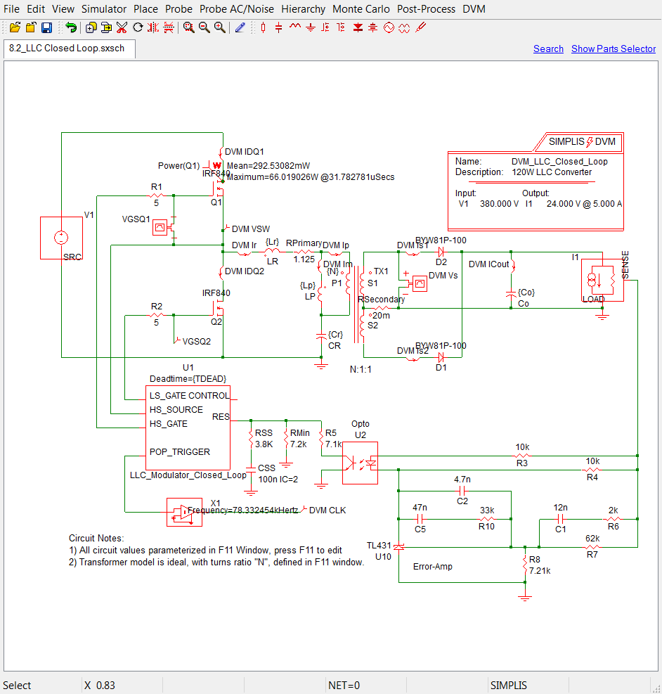
To generate the scalar measurement of the converter switching frequency, a probe with the name DVM CLK is placed on the schematic and connected to the POP trigger output. This probe has the fixed probe measurement "Frequency" applied and will generate a the scalar named "Frequency(CLK)" with the value measured from the simulation. Using the testplan Alias function, we create three scalar measurement aliases for each scalar, one for each line voltage. Finally, after all simulations complete, we generate summary curves using the CreateXYScalarPlot function. As with the example is section 8.1, we use a postprocess script to and use the SIMetrix script version of CreateXYScalarPlot, which is SimplisDVMAdvancedUtilMeasurementCreateXYScalarPlot.
The testplan for this example is shown below. This testplan contains Bode Plot tests at Load levels from 5% to 100% of full load and at three input voltages, Minimum, Nominal, and Maximum. As with the example in section 8.1, this testplan uses 5% load steps from 5% to 40% of full load, and 10% load steps from 40% to 100% of full load. The final summary curves are generated from five different tests, allowing for easy report customization.
| *** | |||||||||||
|---|---|---|---|---|---|---|---|---|---|---|---|
| *** 8.2_efficiency_and_loop_characteristics.testplan | |||||||||||
| *** | |||||||||||
| *** | |||||||||||
| *?@ analysis | objective | source | load | label | Measurement | Measurement | Measurement | Measurement | Measurement | Measurement | postprocess |
| *** | |||||||||||
| Ac | BodePlot(OUTPUT:1) | SOURCE(INPUT:1, Nominal) | LOAD(OUTPUT:1, 5%) | Efficiency and Loop Characterization|Vin Nominal|5% Load | alias(Efficiency,eta_nom) | alias(Avg(ILOAD), iload_nom) | alias(gain_crossover_freq, gxover_nom) | alias(gain_margin, gmargin_nom) | alias(phase_margin, pmargin_nom) | alias( Frequency(CLK) , sw_freq_nom ) | |
| Ac | BodePlot(OUTPUT:1) | SOURCE(INPUT:1, Nominal) | LOAD(OUTPUT:1, 10%) | Efficiency and Loop Characterization|Vin Nominal|10% Load | alias(Efficiency,eta_nom) | alias(Avg(ILOAD), iload_nom) | alias(gain_crossover_freq, gxover_nom) | alias(gain_margin, gmargin_nom) | alias(phase_margin, pmargin_nom) | alias( Frequency(CLK) , sw_freq_nom ) | |
| Ac | BodePlot(OUTPUT:1) | SOURCE(INPUT:1, Nominal) | LOAD(OUTPUT:1, 15%) | Efficiency and Loop Characterization|Vin Nominal|15% Load | alias(Efficiency,eta_nom) | alias(Avg(ILOAD), iload_nom) | alias(gain_crossover_freq, gxover_nom) | alias(gain_margin, gmargin_nom) | alias(phase_margin, pmargin_nom) | alias( Frequency(CLK) , sw_freq_nom ) | |
| Ac | BodePlot(OUTPUT:1) | SOURCE(INPUT:1, Nominal) | LOAD(OUTPUT:1, 20%) | Efficiency and Loop Characterization|Vin Nominal|20% Load | alias(Efficiency,eta_nom) | alias(Avg(ILOAD), iload_nom) | alias(gain_crossover_freq, gxover_nom) | alias(gain_margin, gmargin_nom) | alias(phase_margin, pmargin_nom) | alias( Frequency(CLK) , sw_freq_nom ) | |
| Ac | BodePlot(OUTPUT:1) | SOURCE(INPUT:1, Nominal) | LOAD(OUTPUT:1, 25%) | Efficiency and Loop Characterization|Vin Nominal|25% Load | alias(Efficiency,eta_nom) | alias(Avg(ILOAD), iload_nom) | alias(gain_crossover_freq, gxover_nom) | alias(gain_margin, gmargin_nom) | alias(phase_margin, pmargin_nom) | alias( Frequency(CLK) , sw_freq_nom ) | |
| Ac | BodePlot(OUTPUT:1) | SOURCE(INPUT:1, Nominal) | LOAD(OUTPUT:1, 30%) | Efficiency and Loop Characterization|Vin Nominal|30% Load | alias(Efficiency,eta_nom) | alias(Avg(ILOAD), iload_nom) | alias(gain_crossover_freq, gxover_nom) | alias(gain_margin, gmargin_nom) | alias(phase_margin, pmargin_nom) | alias( Frequency(CLK) , sw_freq_nom ) | |
| Ac | BodePlot(OUTPUT:1) | SOURCE(INPUT:1, Nominal) | LOAD(OUTPUT:1, 35%) | Efficiency and Loop Characterization|Vin Nominal|35% Load | alias(Efficiency,eta_nom) | alias(Avg(ILOAD), iload_nom) | alias(gain_crossover_freq, gxover_nom) | alias(gain_margin, gmargin_nom) | alias(phase_margin, pmargin_nom) | alias( Frequency(CLK) , sw_freq_nom ) | |
| Ac | BodePlot(OUTPUT:1) | SOURCE(INPUT:1, Nominal) | LOAD(OUTPUT:1, 40%) | Efficiency and Loop Characterization|Vin Nominal|40% Load | alias(Efficiency,eta_nom) | alias(Avg(ILOAD), iload_nom) | alias(gain_crossover_freq, gxover_nom) | alias(gain_margin, gmargin_nom) | alias(phase_margin, pmargin_nom) | alias( Frequency(CLK) , sw_freq_nom ) | |
| Ac | BodePlot(OUTPUT:1) | SOURCE(INPUT:1, Nominal) | LOAD(OUTPUT:1, 50%) | Efficiency and Loop Characterization|Vin Nominal|50% Load | alias(Efficiency,eta_nom) | alias(Avg(ILOAD), iload_nom) | alias(gain_crossover_freq, gxover_nom) | alias(gain_margin, gmargin_nom) | alias(phase_margin, pmargin_nom) | alias( Frequency(CLK) , sw_freq_nom ) | |
| Ac | BodePlot(OUTPUT:1) | SOURCE(INPUT:1, Nominal) | LOAD(OUTPUT:1, 60%) | Efficiency and Loop Characterization|Vin Nominal|60% Load | alias(Efficiency,eta_nom) | alias(Avg(ILOAD), iload_nom) | alias(gain_crossover_freq, gxover_nom) | alias(gain_margin, gmargin_nom) | alias(phase_margin, pmargin_nom) | alias( Frequency(CLK) , sw_freq_nom ) | |
| Ac | BodePlot(OUTPUT:1) | SOURCE(INPUT:1, Nominal) | LOAD(OUTPUT:1, 70%) | Efficiency and Loop Characterization|Vin Nominal|70% Load | alias(Efficiency,eta_nom) | alias(Avg(ILOAD), iload_nom) | alias(gain_crossover_freq, gxover_nom) | alias(gain_margin, gmargin_nom) | alias(phase_margin, pmargin_nom) | alias( Frequency(CLK) , sw_freq_nom ) | |
| Ac | BodePlot(OUTPUT:1) | SOURCE(INPUT:1, Nominal) | LOAD(OUTPUT:1, 80%) | Efficiency and Loop Characterization|Vin Nominal|80% Load | alias(Efficiency,eta_nom) | alias(Avg(ILOAD), iload_nom) | alias(gain_crossover_freq, gxover_nom) | alias(gain_margin, gmargin_nom) | alias(phase_margin, pmargin_nom) | alias( Frequency(CLK) , sw_freq_nom ) | |
| Ac | BodePlot(OUTPUT:1) | SOURCE(INPUT:1, Nominal) | LOAD(OUTPUT:1, 90%) | Efficiency and Loop Characterization|Vin Nominal|90% Load | alias(Efficiency,eta_nom) | alias(Avg(ILOAD), iload_nom) | alias(gain_crossover_freq, gxover_nom) | alias(gain_margin, gmargin_nom) | alias(phase_margin, pmargin_nom) | alias( Frequency(CLK) , sw_freq_nom ) | |
| Ac | BodePlot(OUTPUT:1) | SOURCE(INPUT:1, Nominal) | LOAD(OUTPUT:1, 100%) | Efficiency and Loop Characterization|Vin Nominal|100% Load | alias(Efficiency,eta_nom) | alias(Avg(ILOAD), iload_nom) | alias(gain_crossover_freq, gxover_nom) | alias(gain_margin, gmargin_nom) | alias(phase_margin, pmargin_nom) | alias( Frequency(CLK) , sw_freq_nom ) | |
| *** | |||||||||||
| Ac | BodePlot(OUTPUT:1) | SOURCE(INPUT:1, Maximum) | LOAD(OUTPUT:1, 5%) | Efficiency and Loop Characterization|Vin Maximum|5% Load | alias(Efficiency,eta_max) | alias(Avg(ILOAD), iload_max) | alias(gain_crossover_freq, gxover_max) | alias(gain_margin, gmargin_max) | alias(phase_margin, pmargin_max) | alias( Frequency(CLK) , sw_freq_max ) | |
| Ac | BodePlot(OUTPUT:1) | SOURCE(INPUT:1, Maximum) | LOAD(OUTPUT:1, 10%) | Efficiency and Loop Characterization|Vin Maximum|10% Load | alias(Efficiency,eta_max) | alias(Avg(ILOAD), iload_max) | alias(gain_crossover_freq, gxover_max) | alias(gain_margin, gmargin_max) | alias(phase_margin, pmargin_max) | alias( Frequency(CLK) , sw_freq_max ) | |
| Ac | BodePlot(OUTPUT:1) | SOURCE(INPUT:1, Maximum) | LOAD(OUTPUT:1, 15%) | Efficiency and Loop Characterization|Vin Maximum|15% Load | alias(Efficiency,eta_max) | alias(Avg(ILOAD), iload_max) | alias(gain_crossover_freq, gxover_max) | alias(gain_margin, gmargin_max) | alias(phase_margin, pmargin_max) | alias( Frequency(CLK) , sw_freq_max ) | |
| Ac | BodePlot(OUTPUT:1) | SOURCE(INPUT:1, Maximum) | LOAD(OUTPUT:1, 20%) | Efficiency and Loop Characterization|Vin Maximum|20% Load | alias(Efficiency,eta_max) | alias(Avg(ILOAD), iload_max) | alias(gain_crossover_freq, gxover_max) | alias(gain_margin, gmargin_max) | alias(phase_margin, pmargin_max) | alias( Frequency(CLK) , sw_freq_max ) | |
| Ac | BodePlot(OUTPUT:1) | SOURCE(INPUT:1, Maximum) | LOAD(OUTPUT:1, 25%) | Efficiency and Loop Characterization|Vin Maximum|25% Load | alias(Efficiency,eta_max) | alias(Avg(ILOAD), iload_max) | alias(gain_crossover_freq, gxover_max) | alias(gain_margin, gmargin_max) | alias(phase_margin, pmargin_max) | alias( Frequency(CLK) , sw_freq_max ) | |
| Ac | BodePlot(OUTPUT:1) | SOURCE(INPUT:1, Maximum) | LOAD(OUTPUT:1, 30%) | Efficiency and Loop Characterization|Vin Maximum|30% Load | alias(Efficiency,eta_max) | alias(Avg(ILOAD), iload_max) | alias(gain_crossover_freq, gxover_max) | alias(gain_margin, gmargin_max) | alias(phase_margin, pmargin_max) | alias( Frequency(CLK) , sw_freq_max ) | |
| Ac | BodePlot(OUTPUT:1) | SOURCE(INPUT:1, Maximum) | LOAD(OUTPUT:1, 35%) | Efficiency and Loop Characterization|Vin Maximum|35% Load | alias(Efficiency,eta_max) | alias(Avg(ILOAD), iload_max) | alias(gain_crossover_freq, gxover_max) | alias(gain_margin, gmargin_max) | alias(phase_margin, pmargin_max) | alias( Frequency(CLK) , sw_freq_max ) | |
| Ac | BodePlot(OUTPUT:1) | SOURCE(INPUT:1, Maximum) | LOAD(OUTPUT:1, 40%) | Efficiency and Loop Characterization|Vin Maximum|40% Load | alias(Efficiency,eta_max) | alias(Avg(ILOAD), iload_max) | alias(gain_crossover_freq, gxover_max) | alias(gain_margin, gmargin_max) | alias(phase_margin, pmargin_max) | alias( Frequency(CLK) , sw_freq_max ) | |
| Ac | BodePlot(OUTPUT:1) | SOURCE(INPUT:1, Maximum) | LOAD(OUTPUT:1, 50%) | Efficiency and Loop Characterization|Vin Maximum|50% Load | alias(Efficiency,eta_max) | alias(Avg(ILOAD), iload_max) | alias(gain_crossover_freq, gxover_max) | alias(gain_margin, gmargin_max) | alias(phase_margin, pmargin_max) | alias( Frequency(CLK) , sw_freq_max ) | |
| Ac | BodePlot(OUTPUT:1) | SOURCE(INPUT:1, Maximum) | LOAD(OUTPUT:1, 60%) | Efficiency and Loop Characterization|Vin Maximum|60% Load | alias(Efficiency,eta_max) | alias(Avg(ILOAD), iload_max) | alias(gain_crossover_freq, gxover_max) | alias(gain_margin, gmargin_max) | alias(phase_margin, pmargin_max) | alias( Frequency(CLK) , sw_freq_max ) | |
| Ac | BodePlot(OUTPUT:1) | SOURCE(INPUT:1, Maximum) | LOAD(OUTPUT:1, 70%) | Efficiency and Loop Characterization|Vin Maximum|70% Load | alias(Efficiency,eta_max) | alias(Avg(ILOAD), iload_max) | alias(gain_crossover_freq, gxover_max) | alias(gain_margin, gmargin_max) | alias(phase_margin, pmargin_max) | alias( Frequency(CLK) , sw_freq_max ) | |
| Ac | BodePlot(OUTPUT:1) | SOURCE(INPUT:1, Maximum) | LOAD(OUTPUT:1, 80%) | Efficiency and Loop Characterization|Vin Maximum|80% Load | alias(Efficiency,eta_max) | alias(Avg(ILOAD), iload_max) | alias(gain_crossover_freq, gxover_max) | alias(gain_margin, gmargin_max) | alias(phase_margin, pmargin_max) | alias( Frequency(CLK) , sw_freq_max ) | |
| Ac | BodePlot(OUTPUT:1) | SOURCE(INPUT:1, Maximum) | LOAD(OUTPUT:1, 90%) | Efficiency and Loop Characterization|Vin Maximum|90% Load | alias(Efficiency,eta_max) | alias(Avg(ILOAD), iload_max) | alias(gain_crossover_freq, gxover_max) | alias(gain_margin, gmargin_max) | alias(phase_margin, pmargin_max) | alias( Frequency(CLK) , sw_freq_max ) | |
| Ac | BodePlot(OUTPUT:1) | SOURCE(INPUT:1, Maximum) | LOAD(OUTPUT:1, 100%) | Efficiency and Loop Characterization|Vin Maximum|100% Load | alias(Efficiency,eta_max) | alias(Avg(ILOAD), iload_max) | alias(gain_crossover_freq, gxover_max) | alias(gain_margin, gmargin_max) | alias(phase_margin, pmargin_max) | alias( Frequency(CLK) , sw_freq_max ) | |
| *** | |||||||||||
| Ac | BodePlot(OUTPUT:1) | SOURCE(INPUT:1, Minimum) | LOAD(OUTPUT:1, 5%) | Efficiency and Loop Characterization|Vin Minimum|5% Load | alias(Efficiency,eta_min) | alias(Avg(ILOAD), iload_min) | alias(gain_crossover_freq, gxover_min) | alias(gain_margin, gmargin_min) | alias(phase_margin, pmargin_min) | alias( Frequency(CLK) , sw_freq_min ) | |
| Ac | BodePlot(OUTPUT:1) | SOURCE(INPUT:1, Minimum) | LOAD(OUTPUT:1, 10%) | Efficiency and Loop Characterization|Vin Minimum|10% Load | alias(Efficiency,eta_min) | alias(Avg(ILOAD), iload_min) | alias(gain_crossover_freq, gxover_min) | alias(gain_margin, gmargin_min) | alias(phase_margin, pmargin_min) | alias( Frequency(CLK) , sw_freq_min ) | |
| Ac | BodePlot(OUTPUT:1) | SOURCE(INPUT:1, Minimum) | LOAD(OUTPUT:1, 15%) | Efficiency and Loop Characterization|Vin Minimum|15% Load | alias(Efficiency,eta_min) | alias(Avg(ILOAD), iload_min) | alias(gain_crossover_freq, gxover_min) | alias(gain_margin, gmargin_min) | alias(phase_margin, pmargin_min) | alias( Frequency(CLK) , sw_freq_min ) | |
| Ac | BodePlot(OUTPUT:1) | SOURCE(INPUT:1, Minimum) | LOAD(OUTPUT:1, 20%) | Efficiency and Loop Characterization|Vin Minimum|20% Load | alias(Efficiency,eta_min) | alias(Avg(ILOAD), iload_min) | alias(gain_crossover_freq, gxover_min) | alias(gain_margin, gmargin_min) | alias(phase_margin, pmargin_min) | alias( Frequency(CLK) , sw_freq_min ) | |
| Ac | BodePlot(OUTPUT:1) | SOURCE(INPUT:1, Minimum) | LOAD(OUTPUT:1, 25%) | Efficiency and Loop Characterization|Vin Minimum|25% Load | alias(Efficiency,eta_min) | alias(Avg(ILOAD), iload_min) | alias(gain_crossover_freq, gxover_min) | alias(gain_margin, gmargin_min) | alias(phase_margin, pmargin_min) | alias( Frequency(CLK) , sw_freq_min ) | |
| Ac | BodePlot(OUTPUT:1) | SOURCE(INPUT:1, Minimum) | LOAD(OUTPUT:1, 30%) | Efficiency and Loop Characterization|Vin Minimum|30% Load | alias(Efficiency,eta_min) | alias(Avg(ILOAD), iload_min) | alias(gain_crossover_freq, gxover_min) | alias(gain_margin, gmargin_min) | alias(phase_margin, pmargin_min) | alias( Frequency(CLK) , sw_freq_min ) | |
| Ac | BodePlot(OUTPUT:1) | SOURCE(INPUT:1, Minimum) | LOAD(OUTPUT:1, 35%) | Efficiency and Loop Characterization|Vin Minimum|35% Load | alias(Efficiency,eta_min) | alias(Avg(ILOAD), iload_min) | alias(gain_crossover_freq, gxover_min) | alias(gain_margin, gmargin_min) | alias(phase_margin, pmargin_min) | alias( Frequency(CLK) , sw_freq_min ) | |
| Ac | BodePlot(OUTPUT:1) | SOURCE(INPUT:1, Minimum) | LOAD(OUTPUT:1, 40%) | Efficiency and Loop Characterization|Vin Minimum|40% Load | alias(Efficiency,eta_min) | alias(Avg(ILOAD), iload_min) | alias(gain_crossover_freq, gxover_min) | alias(gain_margin, gmargin_min) | alias(phase_margin, pmargin_min) | alias( Frequency(CLK) , sw_freq_min ) | |
| Ac | BodePlot(OUTPUT:1) | SOURCE(INPUT:1, Minimum) | LOAD(OUTPUT:1, 50%) | Efficiency and Loop Characterization|Vin Minimum|50% Load | alias(Efficiency,eta_min) | alias(Avg(ILOAD), iload_min) | alias(gain_crossover_freq, gxover_min) | alias(gain_margin, gmargin_min) | alias(phase_margin, pmargin_min) | alias( Frequency(CLK) , sw_freq_min ) | |
| Ac | BodePlot(OUTPUT:1) | SOURCE(INPUT:1, Minimum) | LOAD(OUTPUT:1, 60%) | Efficiency and Loop Characterization|Vin Minimum|60% Load | alias(Efficiency,eta_min) | alias(Avg(ILOAD), iload_min) | alias(gain_crossover_freq, gxover_min) | alias(gain_margin, gmargin_min) | alias(phase_margin, pmargin_min) | alias( Frequency(CLK) , sw_freq_min ) | |
| Ac | BodePlot(OUTPUT:1) | SOURCE(INPUT:1, Minimum) | LOAD(OUTPUT:1, 70%) | Efficiency and Loop Characterization|Vin Minimum|70% Load | alias(Efficiency,eta_min) | alias(Avg(ILOAD), iload_min) | alias(gain_crossover_freq, gxover_min) | alias(gain_margin, gmargin_min) | alias(phase_margin, pmargin_min) | alias( Frequency(CLK) , sw_freq_min ) | |
| Ac | BodePlot(OUTPUT:1) | SOURCE(INPUT:1, Minimum) | LOAD(OUTPUT:1, 80%) | Efficiency and Loop Characterization|Vin Minimum|80% Load | alias(Efficiency,eta_min) | alias(Avg(ILOAD), iload_min) | alias(gain_crossover_freq, gxover_min) | alias(gain_margin, gmargin_min) | alias(phase_margin, pmargin_min) | alias( Frequency(CLK) , sw_freq_min ) | |
| Ac | BodePlot(OUTPUT:1) | SOURCE(INPUT:1, Minimum) | LOAD(OUTPUT:1, 90%) | Efficiency and Loop Characterization|Vin Minimum|90% Load | alias(Efficiency,eta_min) | alias(Avg(ILOAD), iload_min) | alias(gain_crossover_freq, gxover_min) | alias(gain_margin, gmargin_min) | alias(phase_margin, pmargin_min) | alias( Frequency(CLK) , sw_freq_min ) | |
| Ac | BodePlot(OUTPUT:1) | SOURCE(INPUT:1, Minimum) | LOAD(OUTPUT:1, 100%) | Efficiency and Loop Characterization|Vin Minimum|100% Load | alias(Efficiency,eta_min) | alias(Avg(ILOAD), iload_min) | alias(gain_crossover_freq, gxover_min) | alias(gain_margin, gmargin_min) | alias(phase_margin, pmargin_min) | alias( Frequency(CLK) , sw_freq_min ) | |
| *** | |||||||||||
| NoSimulation | Efficiency and Loop Characterization|Efficiency Summary | ..\scripts\8.2_efficiency_and_loop_characteristics_post_process.sxscr | |||||||||
| NoSimulation | Efficiency and Loop Characterization|Gain Crossover Frequency | ..\scripts\8.2_efficiency_and_loop_characteristics_post_process.sxscr | |||||||||
| NoSimulation | Efficiency and Loop Characterization|Gain Margin | ..\scripts\8.2_efficiency_and_loop_characteristics_post_process.sxscr | |||||||||
| NoSimulation | Efficiency and Loop Characterization|Phase Margin | ..\scripts\8.2_efficiency_and_loop_characteristics_post_process.sxscr | |||||||||
| NoSimulation | Efficiency and Loop Characterization|Switching Frequency | ..\scripts\8.2_efficiency_and_loop_characteristics_post_process.sxscr | |||||||||
LLC/8.2_LLC Closed Loop.sxsch, the overview test report contains the five summary graphs followed by the individual test reports.
8.3 Summary
In Part 2 of this DVM Tutorial, we have shown how to create custom testplans by modifying the built-in testplans. After modifying the schematic to use variables, the testplan functions Var and Globalvar were used to change component values. The Change function was used to change schematic component values directly, without any modifications to the schematic. We also learned how to change the schematic configuration using the jumper testplan entry.
We then learned about the measurement testplan entry which is used for general purpose post-processing . The valid measurement column entries were then covered in detail starting with the Alias function. The Alias testplan entry creates a copy of a scalar measurement with a new name. Once the scalar measurements were aliased, we learned how to create new curves from the aggregated scalar measurements using the CreateXYScalarPlot function. Also useful for comparing test runs is the ExtractCurve function, which creates a copies a curve generated in a previously run test to the current test, allowing direct, visual comparison of multiple curves.
Individual report customizing functions NoSpecs, NoScalars and NoCurves allowed us to change the reported specification, scalar and curve data on a test by test basis. We also learned how to add curves to reports using the ArbitraryCurve and ArbitraryBodePlot functions. Using the overview reporting functions, we learned how to place measured scalar values on the overview report with the PromoteScalar function, while graphs were placed on the overview report with the PromoteGraph function.
The pre and post process script functions discussed with examples shown in the Applications section. We learned how to create and report both user defined specification and user defined scalar values using the SimplisDVMAdvancedUtilCreateSpec and SimplisDVMAdvancedUtilCreateScalar functions.
Finally, we showed a two applications of the Design Verification Module. In these examples, the efficiency, power loss, and control loop behavior across line and load variation was measured, graphed and then saved into an archive quality html report.
© 2013 simplistechnologies.com | All Rights Reserved